Ghosts of Christmas Past: Live Imaging Bead Capture on 0.5 μm Microporous Membranes

The last time I did live imaging on the confocal microscope was in December of 2019. Then I was imaging the capture of 1.24 µm diameter beads in 1 µm slit pore membranes to visualize the difference between steric and affinity based capture. This time around, all of the materials are different, but the process is the same. Recently I withdrew beads onto 0.5 µm microporous membranes to visualize pore patency (described here). While this worked well to show that a majority of the pores on the membrane participate in fluid flow, we wanted to try to take this protocol one step further and count the beads that we captured while reaching 100% capacity. This post describes our initial efforts to do this.

Live Imaging the Capture of 510 nm Diameter Beads on 0.5 µm Microporous Membranes

Our first attempt at live imaging involved the use of 510 nm diameter fluorescent beads and 0.5 µm microporous membranes. Our goal was to capture enough beads to visualize 100% capacity of the membrane. Although troublesome in the past, we first tried withdrawing our bead solutions by hand. Just as it had before, this posed difficult as the position of the µSiM beneath the head of the microscope made the angle that you have to use the pipette at awkward. This often led to issues with the seal between the pipette tip and the port of the device, but more importantly made it nearly impossible to live image since the device often moved around. To avoid this, we used a syringe pump to withdraw our bead solution for us following the protocol described below.

Protocol

To prepare the µSiM-CA for testing, we followed our standard wetting procedure detailed below.

1. Pipette ~15 µL of PBS by inserting the pipette tip into one of the two open ports of the µSiM-CA and depressing the plunger of the pipette; the PBS should flow from this port through the bottom channel and out the opposite, open port. Remove the pipette tip before releasing the plunger of the pipette to avoid sucking injected fluid back out of the bottom channel of the device
2. Fill the well of the µSiM-CA by pipetting 100 µL of fresh PBS into it; care is taken to not create air bubbles and/or remove them by by withdrawing injected media and injecting it again until no air bubbles are visible
3. With the bottom channel and well wet, block one of the open ports using a 3M double-sided tape sticker and stabilize the devices with clamps around its sides
4. In the same manner as above, pipette ~40 µL of PBS into the open port and look to see the well fill with little resistance. If resistance is appreciable, discard the device and prepare a new one
5. Remove all liquid from the well (~140 µL)
6. Next, add 100 µL of the bead solution at a concentration of 2.5E8 beads/mL to the well of each device, withdrawing and injecting the bead solution again if air bubbles are present until they are gone
7. Add 10 uL of PBS to the well
8. Withdraw 100 µL of fluid from the open port, sucking fluid from the well through the membrane into the bottom channel and out the port
9. Image on the confocal microscope

Syringe Pump Setup

To withdraw our bead solution, we would set the syringe pump next to the microscope stage and load a 1 mL syringe with a blunt needle tip inside the holder of the syringe pump. Separately, we would secure the µSiM-CA to a µSiM slide holder using double-sided tape along the bottom of the holder. By pressing the µSiM-CA into the double-sided tape within the holder, the device became secure enough to attach our tubing. To connect the two, we would make connectors out of tubing and a P200 pipette tip cut about two thirds of the way down from the top. In this manner, the opening at the top of the pipette tip would be slightly larger that the outer diameter of the tubing. This allowed us to insert the tubing inside what remained of the pipette tip far enough to make a seal between the tubing and the tip, but not too far where the tubing would be pinched closed. After inserting the tubing, nail polish was used to solidify the connection and ensure the seal between the tubing and the tip was air tight. Using one of these connectors, we would connect the syringe in the syringe pump to the open port of the µSiM-CA by inserting the blunt syringe needle tip inside of the tubing end of the connector and the pipette tip of the other side of the connector inside the open port of the µSiM-CA. Care was taken to make sure the pipette tip was pushed deep enough into the port so that a tight seal was created between the two. With all of this in place, we would set the syringe pump with the following settings:

Flow rate: 100 µL/min

Flow type: Withdrawal

Flow time: 60 seconds

Confocal Scope Setup

We used the 488 nm laser and the 525 filter to image our beads. We also used the time series setup, capturing images at the fastest setting of the scope for 5 minutes or until our entire bead volume was withdrawn.

Results

After starting the withdrawal of our bead solution, we quickly realized that the flow rate was too high to continuously image the membrane while keeping it in focus. Withdrawing at 100 uL/min created enough transmembrane pressure to deflect the membrane substantially. This meant that the focal plane with which we needed to image in was constantly changing as the membrane flexed and bowed back and forth. In spite of this, we were still able to get images of the membrane before withdrawal, during withdrawal, and after withdrawal by stopping active withdrawal in order to keep the membrane from bending. These images are shown below in Figure 1.

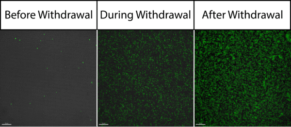
Our images revealed two main things: a) our bead concentration seems close to where we need it to be to in order to reach 100% capacity of the membrane and b) these beads have a tendency to aggregate aggressively. Before addressing these issues, I tried to account for the deflection that we were seeing in the membrane while still using the same protocol and withdrawal settings by using the wide field modality instead of the confocal modality. In this manner, I hoped to keep the beads that were collecting on the membrane in focus throughout the withdrawal process no matter how hard the membrane deflected. Shown in the video below, this did work as intended but it also enabled our fluorescent intensity to reach heights outside of the limitations of our camera. This caused the video to blow out towards the end as the membrane filled with beads.

With two problems to solve (bead aggregation and membrane fluctuation), we moved forward with appropriate adjustments. Seeing that these beads were expired and years old, we decided to order new beads in hopes that they would not aggregate as badly. We also decided to use a slower withdrawal rate in our next attempt to see if we could live image the membrane more effectively in the confocal modality.

Live Imaging the Capture of 860 nm Diameter Beads on 0.5 µm Microporous Membranes

The inter-pore spacing in 0.5 µm Microporous Membranes is ~1 um. With this in mind, we ordered new particles that had a diameter of 860 nm. At 100% capacity, these should be able to fill the membrane while still leaving space in between each particle, allowing for accurate counting using our ComDet ImageJ plugin. Using the same protocol and setup as before, we adjusted a few parameters to fit our new particles a findings, namely: a) we imaged using the 561 nm laser and the 600 nm filter and b) we lowered the withdrawal rate to 60 uL/min to limit membrane deflection. We also changed our bead concentration, each shown before their respective videos below.

Withdrawing 100 uL from a 110 uL 2.5E8 beads/mL solution:

Withdrawing 100 uL from a 110 uL 1.25E8 beads/mL solution:

Withdrawing 100 uL from a 110 uL 2.27E7 beads/mL solution:

Continuing to see an aggregation issue even with these new particles, we decided to try to change our dilution liquid to see if we could limit aggregation. As a result we switched from using PBS to dilute our beads and wet our device to using DI water instead. We also started sonicating our beads for at least a minute just before loading them into the well of our µSiM-CAs. Videos capturing our results are shown below.

Withdrawing 100 uL from a 110 uL 2.5E8 beads/mL solution at 10 uL steps:

Withdrawing 100 uL from a 110 uL 2.5E8 beads/mL solution at 10 uL steps:

In these last two videos it was interesting to see that every time we stopped withdrawing with the syringe pump, our captured beads would release back off of the membrane. We had not seen this before and attributed this to a bad seal between the pipette tip and the port of the uSiM.

In all of the videos, we can see that there are still issues with membrane deflection while withdrawing at 60 uL/min. Deflection is much lower than when we withdrew at 100 uL/min, but nonetheless still present. As a temporary fix, we switched back to taking still images. This time we focused on taking images after we withdrew our entire bead solution. These results are shown in Figure 2 below.

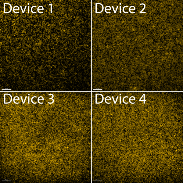
Figure 2 shows that as we had previously thought with our 510 nm beads, 100% membrane capacity seems close to 2.5E7 total beads. There is still aggregation present on the membrane, but a majority of the beads seem unaggregated. Interestingly, being so close to 100% capacity and seemingly having something close to a monolayer of beads on the membrane allows us to see the hexagonal pattern of the pores on the membrane. Ultimately, this emboldened us to try to count the beads that we had captured while continuing to improve the capture process further down the line.

Ensuring Beads are not Pulled Through the Membrane

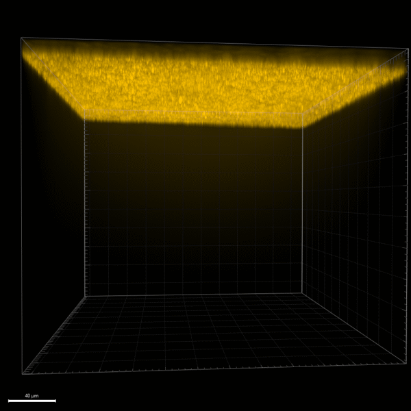
While trying all of these different capture methods and bead concentrations, we anticipated it would be important for future applications to prove that we were not pulling any beads through the membrane with our withdrawal process. To do this, I imaged a large stack of the µSiM-CA containing the membrane and the bottom channel of the device after one of our bead capture experiments. If beads had been pulled through into the bottom channel, we would see them there. Shown in Figure 3 below, we did not, therefore we can reasonably say that this is not a concern with our withdrawal method and polystyrene beads that are ~800 nm in diameter.

Counting 860 nm Diameter Beads on 0.5 µm Microporous Membranes

Now understanding that our beads are in their best condition diluted in water and sonicated before withdrawal, we captured beads from three different concentrations in order to test our counting capabilities. Figure 4 shows the resulting images after withdrawing 100 uL of beads from a total well volume of 110 uL at 10 uL steps.

We chose to image three different bead concentrations around the 2.5E8 bead/mL mark that we previously determined was near 100% capacity of the membrane. The first was 5E8 beads/mL which we knew was over 100% capacity. The second was 2.75E8 beads/mL which we thought would put us even closer to 100% capacity. The last was 5E7 beads/mL which we knew would be lower than 100% capacity. Picking these three concentrations allowed us to test the performance of our counting plugin above, near, and below 100% capacity. Our counting results are shown in Figure 5 below and are not particularly inspiring.

Panel a shows us that our counting plugin seems to be hitting its saturation point with our top two concentrations. Despite our highest bead solution having double the amount of beads as our middle bead solution, both had similar counting outputs. This can be attributed to the fact that each solution goes over 100% capacity, therefore most likely creating more than a monolayer of beads on the membrane. It is expected that any counting plugin would struggle in this scenario, so I also plotted the counts for each concentration to independently compare how many beads we counted to how many beads we should have captured according to the volume of beads we had withdrawn at that time. Both of our highest concentration solutions together only had one data point before they each reached 100% capacity that was not at 0 uLs. Relative to all of the rest of their data points, this one was the closest to being what we expected. After 100% capacity, bead counts seem to plateau and are not close to being accurate. This is in line with the fact that any bead capture past 100% capacity forms a multilayered cake which is challenging to count with any plugin. The more interesting data to analyze is our lowest concentration bead solution. Here we can see we have many data points below 100% capacity. Unfortunately, our counts are not particularly accurate. This suggests we still have some aggregation issues to address among other things.

Conclusions

While we got the beads in a better state to be counted, our results seem to suggest that a) we have not worked out all of our issues to make counting below 100% capacity accurate and b) counting above 100% capacity is challenging and mistake prone. Moving forward, we will continue to alter factors which may make the beads less aggregated and decrease the amount of membrane bowing during our live imaging. This will increase the quality of our images and ultimately increase the accuracy of our counting. We could also find particles which are smaller than 860 nm. At 100% capacity this will provide greater contrast between particles captured in our hexagonal array, further increasing counting accuracy.