ECMO: Results and Conclusions
After several months of modeling, experimenting, thinking and rethinking, it’s finally time to talk about the conclusions we can draw about nanomembrane ECMO. These conclusions take into account only blood oxygenation, and not blood decarboxylation, which is a different therapy that I have not modeled. You can find my description of the model here, and my report of experimental validation of this model here.
The rationale behind nanomembrane ECMO is that the thinness of nanomembrane should enhance transmembrane transport of oxygen into oxygen-unsaturated blood relative to similar therapies that employ traditional (thick) hollow fiber polymer membranes. The advantage of this in my mind is reduced device size, i.e., a smaller area of membrane enabling a reduction in extracorporeal blood volume. Reduced volume translates directly to reduced blood transfusion volume and frequency, and in turn translates into reduced risk for the patient (and the risk is tremendous).
First in this post I will give due diligence to some technical aspects of the results I’m reporting; then, I’ll get to the good stuff. Skip the first block below if you’re only interested in my results. Skip the second as well if you’re only interested in my conclusions.
In order to answer the question of whether nanomembrane ECMO is feasible, I sought to control for every relevant variable possible and to evaluate the influence of each on the oxygen flux through the membrane. In this work, I report oxygen flux values averaged over the entire membrane area, as it is not constant — it looks something like this:
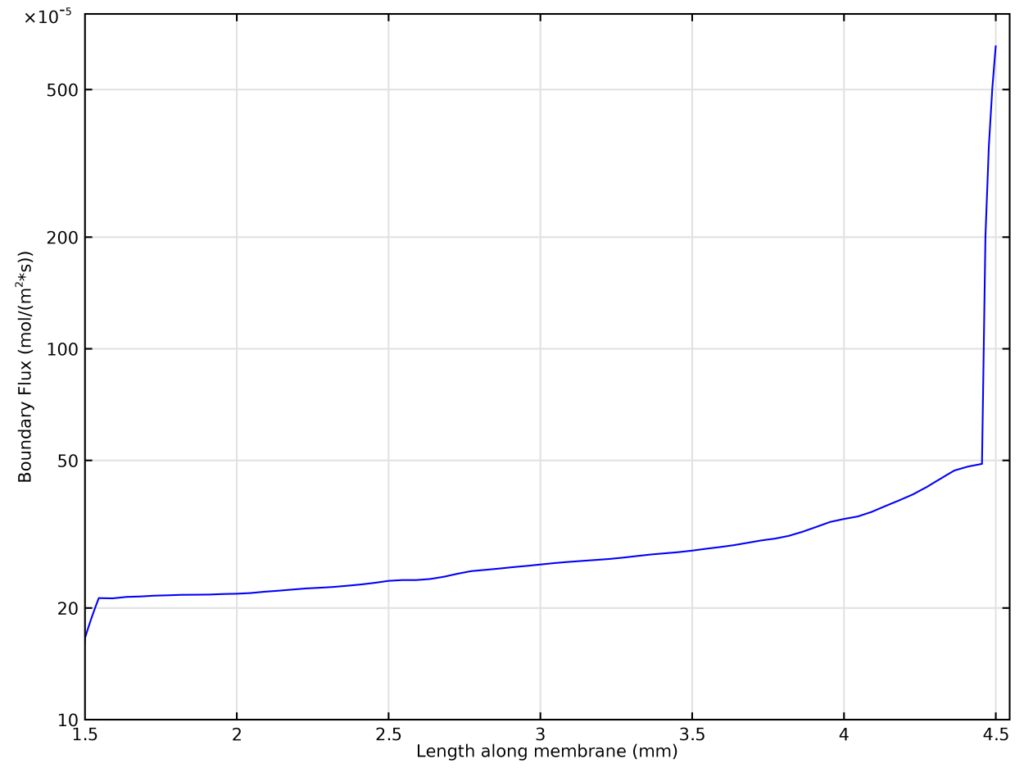
In this figure, absolute oxygen flux across the 3-mm-long membrane is plotted as a function of position along the membrane. The flow originates on the right and goes towards the left. While there’s a huge initial spike in flux at the leading edge of the membrane (notice the logarithmic scale), it quickly falls off and approaches a constant value as the layer of blood adjacent to the membrane rapidly becomes saturated with oxygen and the oxygen concentration gradient becomes smoother (it is initially a step function). This means that the oxygen fluxes reported here will not quite scale linearly with membrane area — at larger membrane areas, the influence of the leading edge will be diminished, and the total average flux across the membrane area will be lower.
Furthermore, it takes some time for the system to reach steady state. I’m not interested in transient behavior (steady state occurs within a few seconds of real time, though that means a few hours of computational time) so all the values I report are for systems that have reached steady-state oxygen flux. I define this by the obvious change in shape on the flux-vs-time plots:

Four different simulations are shown here, each with a different average blood velocity (from top to bottom: 100, 10, 1, and 0.1 mm/s). Before steady-state is achieved, the flux drops logarithmically (this is a log-log plot, so this behavior appears as a straight line) and then once steady-state has been achieved the flux is constant in time. In this plot the 0.1 mm/s simulation has not reached steady state. The odd peaks in flux on these lines are simply transient numerical errors that happened to be taking place as the solver was sending output to the solution.
Okay, so onto the meat of the thing.
I identified three variables that impact oxygen flux in ECMO: the gas phase pressure, the blood flow velocity, and the membrane thickness. Simplifying the system in this way leaves out some nuance — for instance, I don’t control for variation in blood hemoglobin concentration across patients, nor do I take into account the varying membrane diffusion coefficient of oxygen as membrane characteristics change — but I have done my best to ensure that those details which are left out are minor enough to not affect my conclusions.
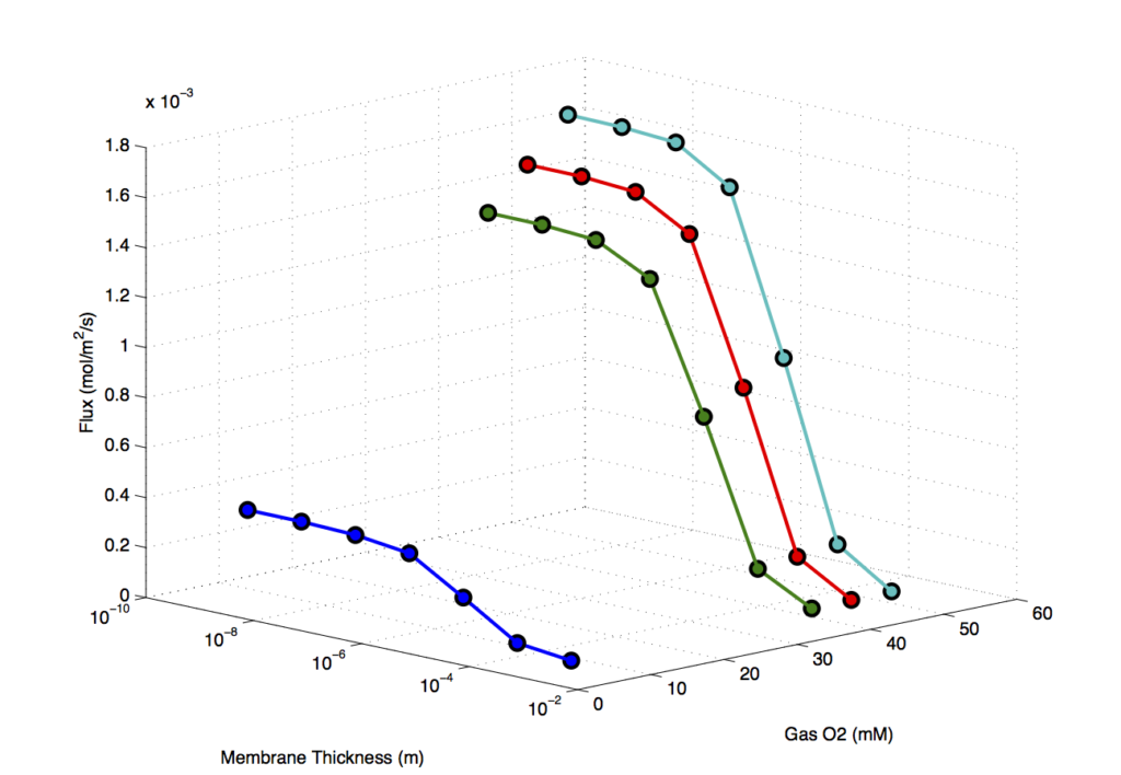
The first and simplest variable is gas phase pressure. It’s intuitive that when the oxygen pressure across the membrane increases, so too should the oxygen’s tendency to travel across the membrane. For fixed membrane thickness and average blood velocity, the relationship between partial oxygen pressure and flux is linear; however, its slope depends on the membrane thickness and average blood velocity.
We can take advantage of this linearity to condense the number of variables we need to think about at once. Suppose we trace lines between each of the points in the above figure according to equal membrane thickness rather than equal concentration of oxygen. Seven straight lines are obtained whose slopes represent the flux per unit of oxygen concentration at varying membrane thicknesses. By taking these slopes as our new dependent variable and plotting them as a function of membrane thickness, we in essence condense the oxygen concentration axis without loss of information:
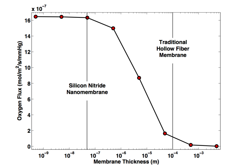
This figure captures the competition between two aspects of the physics: a parabola representing the rate of transport through the membrane versus thickness (average diffusion time goes as the square of diffusion distance) is cut short at the left with an asymptote as transport through the membrane becomes extremely quick relative to transport away from the membrane by diffusion, convection, and reaction. Described in more detail, one can imagine a mass balance of oxygen in the layer of blood adjacent to the membrane: it’s fed by gas coming through the membrane and depleted by diffusion and convection away from it, and also by consumption of the gas by hemoglobin. On the right half of the figure, the rate of oxygen removal from this space is considerably larger than the rate of introduction into it, so membrane diffusion dominates and we see the corresponding parabola. On the left half, the maximum rate of oxygen into this space that the membrane will allow is larger than the rate of depletion, and the flux is limited by the ability of the transport and reaction within the blood to replenish the gradient — a process entirely independent of the membrane thickness. The middle of the plot is a transition region where the rates are comparable to one another.
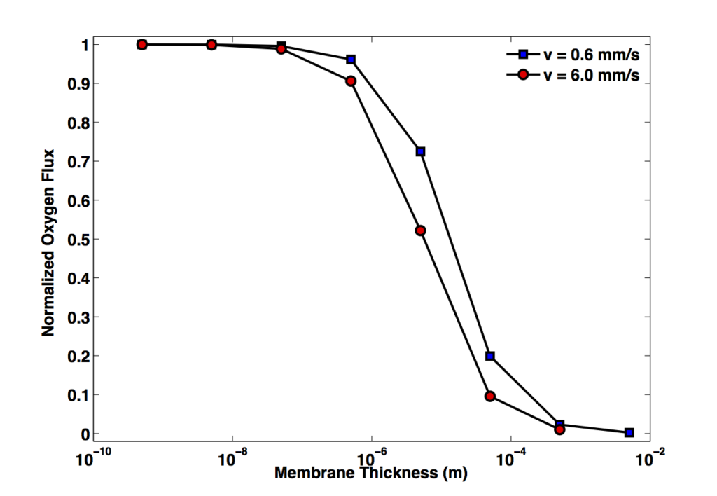
In this light, it is intuitive that a change in the parameters which govern oxygen depletion from the region near the membrane should shift the balance of the curve and change the membrane thickness required to observe asymptotic behavior. For instance, increasing velocity not only promotes convective transport of oxygen away from the membrane, but also brings with it more unsaturated hemoglobin, speeding reaction as well. I am investigating the magnitude of this effect presently, but suffice it to say for now that any membrane thickness could be used to perform at the asymptote, given a sufficiently small blood velocity; it will have to come down to a consideration of whether the required velocity is practical. It appears I accidentally stumbled upon the appropriate velocity for ideal behavior of nanomembranes with my experimental conditions. I’m laying out further experiments now to confirm that I am, in fact, psychic.
EDIT 5/28/16: I now have simulation data to back up the theory in the above paragraph. I would’ve liked to see what happens for both faster and slower velocities, but these simulations take a long time and faster flow rates make them take even longer (decided to cancel my 60 mm/s simulation after two days straight of simulation time only brought it to 4% completion.) The conclusion is that the asymptote does indeed shift, but not all that much given the large change in velocity. Nanomembranes remain useful in the face of this potential criticism.
So what exactly is the effect of velocity? This effect is not so easy to wrangle as the previous two parameters — because it modulates at least three distinct but interrelated aspects of the physics (rate of regeneration of the oxygen gradient; availability of unsaturated heme near the membrane; residence time of blood in channel) it must be understood somewhat more empirically. Furthermore, as the tool we have here (i.e., the model) requires immense computational resources to arrive at solutions, the velocity can only be interrogated to a certain point before it imposes gradients too steep to handle practically.
Holding oxygen pressure constant at 100 mmHg gage and membrane thickness at 50 nm, we see a kind of dull influence of velocity:
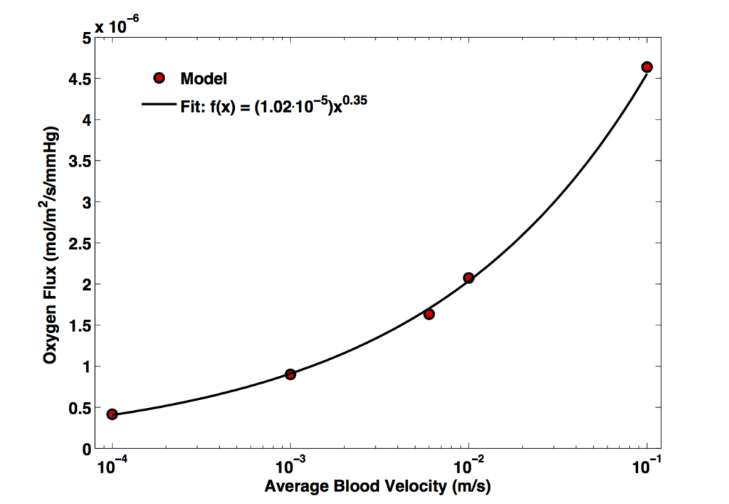
Notice the dissonance in scale: over four orders of magnitude in velocity we get only about one order of magnitude change in flux. The fact of the power law fit makes me a little uncomfortable because I can’t rationalize it to myself (a power law is almost always unphysical, since the units of the independent variable get mutilated by the exponent), but it’s too close a fit not to include (R-squared 0.9991) and might be useful.
It stands to reason that as the velocity increases the flux should increase in response to the steeper concentration gradient, but obviously this behavior cannot continue forever — at some point the oxygen concentration in the blood next to the membrane is effectively equal to its pre-oxygenation level at all times and the flux reaches a max asymptotically. Unfortunately, I can’t find this max because such large velocities are too taxing for even our superpowered Mac Pro — but we can at least rest assured that such questions are academic more than they are practical, since if the velocity is so high that there is no oxygen accumulating in the blood then obviously the oxygenator is a poor one for the purpose! The effect of very high (or very low) velocities could be more easily interrogated by making changes to the membrane size (again, 3 mm long here) such that the residence time of blood at the membrane is being changed for constant velocity, but such things would surely take too long and not be useful or interesting enough for me at this time.
So, is nanomembrane ECMO feasible? Does it do what we want it to do — namely reduce device blood volume below ~1/10 of a neonates blood volume of about 250 mL? The short answer, to anyone who knows our material, is ‘no’. Just about the best device I can design with the information I have includes active membrane area of 0.17 square meters, which is a huge improvement over the two or so square meters of a traditional hollow fiber oxygenator but at the cost of fragility and expensiveness, not to mention the difficulties with fabrication.
More generally and with a bit of spin to it, however, there might be something worth letting the world in on here. Hollow fiber membranes typically have inner diameters of about 200 um; replacing these membranes with our own in the same geometry, only 8.5 mL of blood are required to fill the oxygenator. Compare this to 40 mL employing 0.38 square meters membrane area for the current best option from Maquet (QUADROX-i Neonatal). ‘Geometry matching’ of this type is not strictly fair because our membranes cannot be made into tubes, but it may be useful nonetheless to employ comparisons such as these to emphasize the very real advantage thin membranes could offer. Maybe some day this will really become practical and all this work will help someone!