How a Nanomembrane Prefilter can Enhance Electrophoretic Sensor Capture Under Flow (Part 1)
[latexpage]
This will be at least a three part series. Here in Part I, we will establish why adding flow to electrophoretic sensor (ssNP) is a bad idea. In Part II we will show why microfluidics is a benefit to adhesion-based sensors. In Part III we will explore the ability of a NPN/ssNP dual membrane sensor to overcome the problem explained in Part I.
Electrophoresis
The electric potential in the vicinity of a ssNP is given by …
\begin{equation}
V(r) = \frac{d^2}{8lr} \Delta{V}
\end{equation}
where d is the nanopore size, l is the thickness of the membrane and r is the (radial) distance from the pore and 

The local E field can be found from the derivative of the potential …
\begin{equation}
E(r) = \frac{d^2}{4lr^2} \Delta{V}
\end{equation}
The electrokinetic drift velocity is given by …
\begin{equation}
\italics{v_e(r)} = \mu_b E(r)
\end{equation}
where 
Convection
The velocity profile between two parallel plates separated by a height h is given by ….
\begin{equation}
\italics{v_c(y)} = – \frac{\Delta P h^2}{L•2\mu}\frac{y}{h}(1-\frac{y}{h})
\end{equation}
Which can be recast using the relationship for a steady volumetric flow rate Q, in a rectangular channel …
\begin{equation}
\italics{Q} = \frac{\Delta P h^3•\omega}{12 \mu L }
\end{equation}
as
\begin{equation}
\italics{v_c(y)} = {6\frac{\italics{Q}}{h•\omega}\frac{y}{h}(1-\frac{y}{h})
\end{equation}
Now, if tangential flow is applied to the top of a ssNP sensor it can only be beneficial if the lateral drift due to convection does not exceed the drift toward the sensor due to electrophoresis. Since the electrophoretic drift is largest at the nanopore and falls to zero moving into the bulk while the convective drift starts at zero at the surface and increases toward the bulk, there must be a ‘crossover’ distance at which …
\begin{equation}
\italics{v_c(y*)} = \italics{v_e(r*)}
\end{equation}
where r* = y* is this critical distance measured along the vertical axis in either system.

To find this point directly above the nanopore, let r = y = y* and substitute Equation 2 into Equation 3:
\begin{equation}
E(y*) = \frac{d^2}{4Ly*^2} \Delta{V}
\end{equation}
\begin{equation}
\italics{v_e(y*)} = \mu_b E(y*) = \mu_b \frac{d^2}{4Ly*^2} \Delta{V}
\end{equation}
\begin{equation}
\italics{v_e(y*)} = \mu_b \frac{d^2}{4Ly*^2} \Delta{V} = {6\frac{\italics{Q}}{h•\omega}\frac{y*}{h}(1-\frac{y*}{h}) = \italics{v_c(y*)}
\end{equation}
\begin{equation}
A = \frac{\mu_b d^2 \Delta{V}}{4L}, B = \frac{6Q}{h^2 \omega}
\end{equation}
\begin{equation}
\italics{v_e(y*)} = \frac{A}{y*^2} = By(1-\frac{y*}{h}) = \italics{v_c(y*)}
\end{equation}
\begin{equation}
y*^3(1- \frac{y*}{h}) = \frac{A}{B}
\end{equation}
\begin{equation}
(y*)^3(1- \frac{y*}{h}) = \frac{A}{B} =\mu_b \frac{ d^2h^2 \omega}{24QL}\Delta{V}
\end{equation}
If we make the assumption that the crossover point (y*) is much less than the channel height (h), a direct expression for y* as a function of flow rate is possible:
\begin{equation}
(y*)^3(1-0) = \frac{A}{B} =\mu_b \frac{ d^2h^2 \omega}{24QL}\Delta{V}
\end{equation}
\begin{equation}
y* =\sqrt[3]{ \frac{A}{B}} = \sqrt[3]{\mu_b \frac{ d^2h^2 \omega}{24QL}\Delta{V}}
\end{equation}
where 


From this equation, we can see that the crossover point is inversely related to the flow rate Q; as the convective velocity increases, the crossover point diminishes. Given some typical microfluidic dimensions that we work with, and a typical nanopore geometry, we can estimate this height.
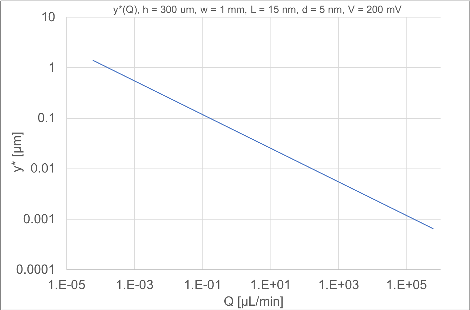
A really high flow rate (1 mL/min) at this scale reduces the crossover point to about 10 nm. For our typical flow rates at (~1-100 uL/min), the crossover point is between 30 nm and 10 nm. This number should be compared to the capture radius for a working ssNP as given by …
\begin{equation}
r* = \Delta{V}\frac{d^2 \mu}{8LD}
\end{equation}
Where D is the diffusion coefficient of DNA in free solution. Consulting the following graph from [3] …

\begin{equation}
log D = m [log(N)]+log(b)
\end{equation}
\begin{equation}
log(D) = -.57 [log(N)]+log(b)
\end{equation}
\begin{equation}
D = 10^{-.57[ log(N)]+log(45e-9)}
\end{equation}
For 1 kbp, D = 45e-9 


For a given size of DNA we can find the point of intersection with the crossover point. To the left of this intersection, flow should not interfere with capture. Above the blue line, it will hamper or preclude it. The highest flow rate possible occurs for the smallest DNA molecule considered (~1 kbp) and is still only 50 nL/min. A proof will be left to Part 2, but such a low flow rate is not going to help overcome the diffusion-limited delivery of molecules to a working ssNP.
So the reason tangential flow microfluidics will not be effective when used to deliver molecules to a ssNP, is because even a mild amount of flow exponentially diminishes the ability of the nanopore to attract molecules; the convective rates of flow dragging molecules past the sensor are much higher than the electrophoretic flows dragging molecules to it, even very near the sensor surface.
[1] Wanunu, M.; Morrison, W.; Rabin, Y.; Grosberg, A. Y.; Meller, A., Electrostatic focusing of unlabelled DNA into nanoscale pores using a salt gradient. Nature nanotechnology 2010, 5 (2), 160-5.
[2] Grosberg, A. Y.; Rabin, Y., DNA capture into a nanopore: interplay of diffusion and electrohydrodynamics. J Chem Phys 2010, 133 (16), 165102.
[3] Nkodo, A. E.; Garnier, J. M.; Tinland, B.; Ren, H.; Desruisseaux, C.; McCormick, L. C.; Drouin, G.; Slater, G. W., Diffusion coefficient of DNA molecules during free solution electrophoresis. Electrophoresis 2001, 22 (12), 2424-32.
This all seems consistent with expectations so far. My question going forward, which I assume you plan to address in a later section, is why NPN can overcome this: while it’s true that you have stagnant liquid between the two membranes, we still need molecules to be captured above the NPN, where flow is happening. But here at the NPN, the voltage drop \Delta V is so much smaller than at the pore (maybe 1% of the applied voltage) that the crossover distance for capture at the NPN layer will be even smaller, and so even the tinest flow will stop DNA from being able to pass through the NPN and into the stagnant space entirely.
To get this working we’ll need to play with the idea of an independent electrode between the two membranes so that the voltage drop at the NPN can be tuned independently from that of the sensing pore. This should be possible with a metal layer in between the oxide spacer and the NPN. Maybe the guys at Simpore could start thinking about ways to realize this on the wafer scale.