Attempting to Quantify Protein Loss to CytoVu Assemblies

As I mentioned in my last post, I will be performing protein diffusion tests through CytoVu assemblies (from one well to the other) and measuring the amount of protein that is still in solution when the system reaches equilibrium in order to determine the amount of protein that is adsorbed to the assembly and thus effectively removed from the system.

The diffusion is occurring now (I’ll be giving the assembly roughly 24 hours to reach equilibrium — this is in keeping with Jessica Snyder’s work with similar tests) but while that’s going on I spent some time preparing to analyze the results. In order to glean the concentration of Cytochrome C in the wells after diffusion, I need to know what type of absorbance to expect from known concentrations. Thus, I analyzed the absorbance spectra of some known concentrations of Cytochrome C in 1x PBS and normalized the data such that pure PBS represented zero absorbance. The spectra are as shown:

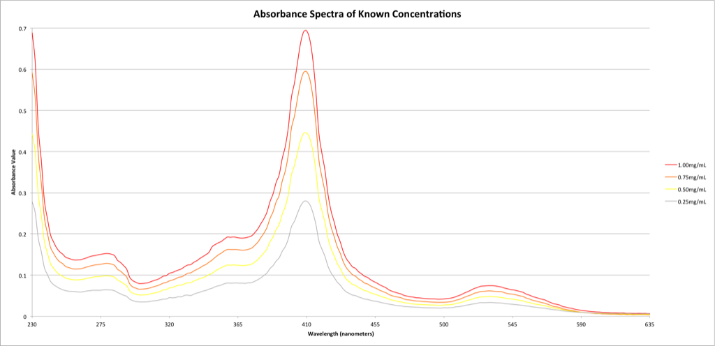
These results are pleasantly predictable, with a clear peak at 410nm. Given this peak, I plotted the absorbance value versus concentration at only 410nm:

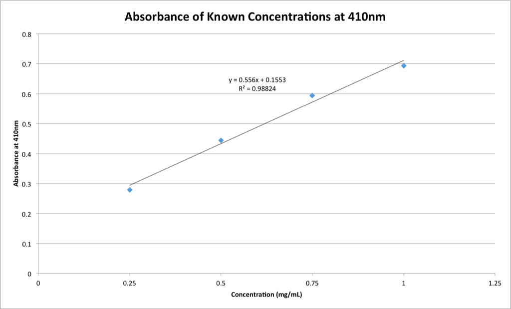
This lovely line will be used to extrapolate the concentrations of the samples taken from the wells of the CytoVu assemblies once the diffusion has reached equilibrium. Since all the volumes are known, I’ll be able to use this concentration to quantify exactly how much adsorption took place during the 24 hours of diffusion.

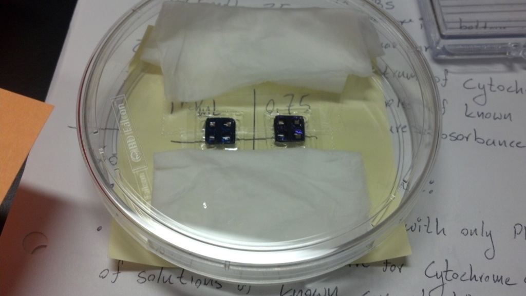
As for the actual diffusion tests, I’ve placed two plasma-bound CytoVu assemblies in a petri dish, stuck to the bottom with double-sided tape to keep them stationary and in order to allow me to be sure of the orientation. The chips themselves are MP8NP50 hybrids, which are two layers of 8um SiN pores sandwiching 50nm pnc-Si pores — ideally, this should not hinder the diffusion of Cytochrome C, which has a diameter of 4.24 ± 0.96nm according to Jessica Snyder’s diffusion paper. On the back of the petri dish I attached a sticky note noting the contents of each well: I’m testing 0.25, 0.5, 0.75, and 1 mg/mL Cytochrome C solutions. Finally, I folded up two Kimwipes and wet them with DI water before placing them in the petri dish and shutting the lid. This is to wet the ambient air in order to negate the evaporation of water from the systems, which could have an obvious effect on the results of the experiment.

Tomorrow, then, I should have the results of the test. Hopefully the protein adsorption will be very low, but only time will tell. I’ll update this post with the results of my analysis of tomorrow’s data when I have it.

UPDATE: The data are in! Today I took 3uL samples from every bottom well, as well as from four of the top wells, and analyzed their absorbance at 410nm with the TECAN.

To be safe, I took new absorbance data for the stock solutions, and plotted them in the same way as before. Comfortingly, it’s similar today to yesterday’s graph:

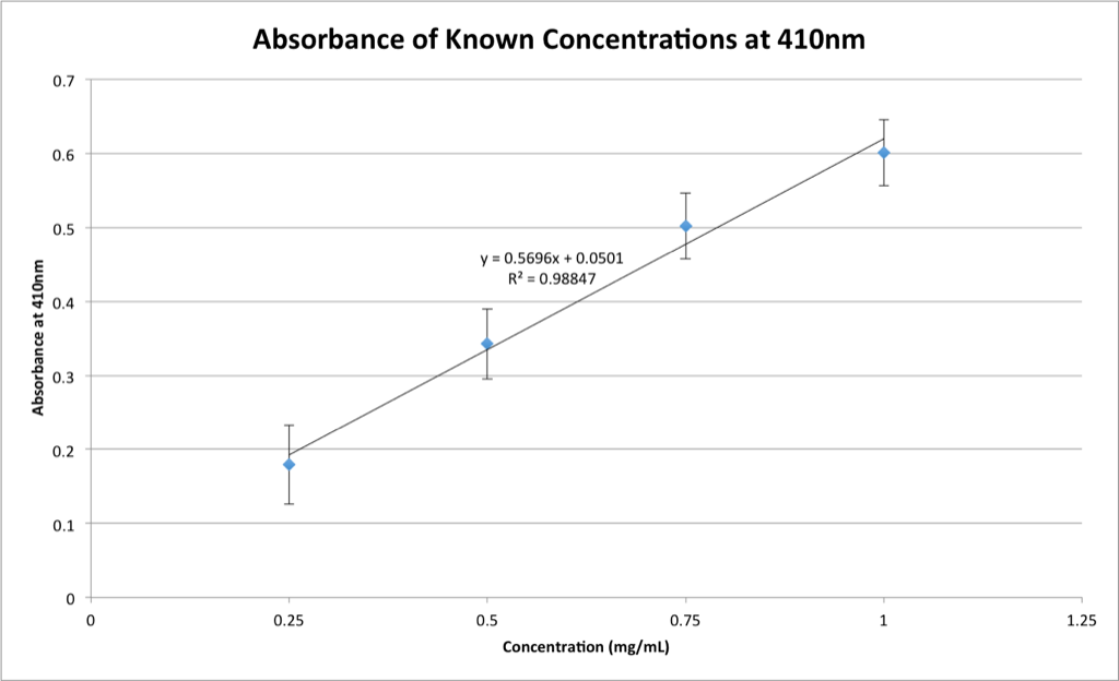
This time, I took nine measurements of each sample in order to determine a standard deviation for the absorbance values. Using this linear regression, I calculated the concentrations of Cytochrome C in each of my samples from their absorbance values, and compared these values to “ideal” concentration values scaled to the new volume of the system (34.3uL up from 9.3uL.) The difference between actual and ideal concentration represents the amount of protein adsorbed to the system, after accounting for measurement and experimental error. Difference is positive for concentrations which are higher than expected.

	Absorbance	Concentration (Measured) (mg/mL)	Concentration (Measured) (uM)	Concentration (Ideal) (mg/mL)	Concentration (Ideal) (uM)	Difference (mg/mL)	Difference (uM)
Left 1mg/mL	0.23	0.32	26.2	0.270	21.9	0.05	4.27
Right 1mg/mL	0.22	0.29	23.5	0.270	21.9	0.02	1.61
Left 0.75	0.14	0.16	12.7	0.203	16.4	-0.05	-3.77
Right 0.75	0.12	0.13	10.6	0.203	16.4	-0.07	-5.87
Left 0.5	0.12	0.13	10.6	0.135	11.0	0.00	-0.37
Right 0.5	0.12	0.13	10.5	0.135	11.0	-0.01	-0.50
Left 0.25	0.09	0.07	5.58	0.068	5.48	0.00	0.11
Right 0.25	0.09	0.07	5.80	0.068	5.48	0.00	0.32
Left 1.0 Top	0.24	0.33	26.8	0.270	21.9	0.06	4.90
Right 1.0 Top	0.24	0.34	27.3	0.270	21.9	0.07	5.46
Left 0.5 Top	0.15	0.17	13.8	0.135	11.0	0.04	2.88
Right 0.5 Top	0.14	0.17	13.4	0.135	11.0	0.03	2.45

All-in-all, these are pretty small values and are easily explained by measurement error alone — when the absorbance values are taken to be the mean plus one standard deviation, instead of simply the mean as shown here, the difference values are more than an order of magnitude larger on average (0.21mg/mL, up from 0.1mg/mL.) It seems that, at worst, a few ug of Cytochrome C are lost to the system.

Finally, it’s worth noting that while it is possible for the samples taken from the top wells to have actual concentrations higher than anticipated, the same is not reasonably possible for samples taken from the bottom well — that would imply that the diffusion went significantly past equilibrium, or else that Cytochrome C was added to the system. More likely, some combination of measurement error and slight evaporation probably led to those values.

UPDATE: As per my conversation with Jim, I’ll provide a bit more information. I’ve updated the above table to include concentrations in uM using the molecular mass of Cytochrome C as a conversion factor, and below I’ll report on the accuracy of measurements.

As the concentration of Cytochrome C in the sample gets lower, the standard deviation grows exponentially. Using nine measurements for each of my four samples, I plotted the Standard % Error ([Standard Deviation/Average Value] * 100) of the concentration versus the concentration for known-concentration samples.

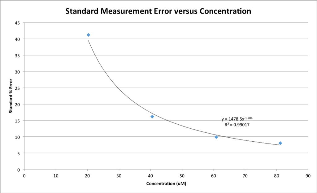
Error reaches slightly over 40% for the 20uM samples. More accurately, it’s about 7.6uM of error. Given the near-zero mean Cytochrome C loss for 20uM samples, then, I feel confident saying that a concentration change of no more than about 8uM took place in these samples. Once the starting concentration reaches about 40uM, the error becomes as small as 16% of the average, or 6.7uM, and the 60uM and 80uM samples are both similar at 6.3uM.

Overall, a concentration change on the order of 10uM — About 3.4nMol — is the most that can be expected. It will have to be determined whether or not this is acceptable for assays, or if effort should be put towards applying surface modifications such as PEG and DDM in an effort to increase the assay’s sensitivity.

In any event, a big next step in the proof-of-concept here will be proving that the assay will block large molecules while permitting smaller ones. I believe Jamie mentioned that the best option for proving this might be FLAG and Anti-FLAG molecules, so if all goes well I’ll be attempting those tests and making a new post with the results in the near future.