Why Flow Benefits Adhesion Based Sensors
[latexpage]
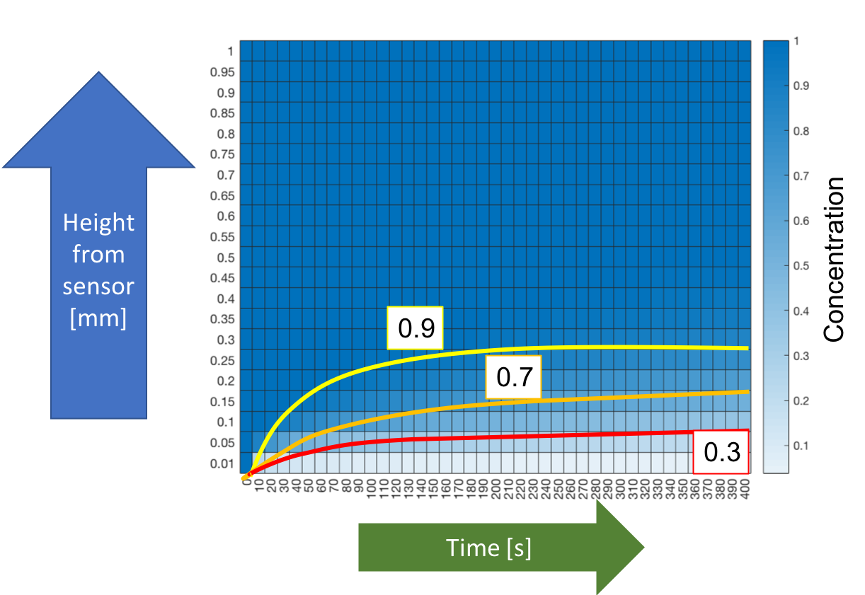
The solution to the problem of diffusion from a semi-infinite solution to a perfectly absorbing surface is found on page 32 of Crank’s classic text (The Mathematics of Diffusion):
\begin{equation}
\frac{C(y,t)}{C_o} = erf(\frac{y}{2\sqrt{Dt}})
\end{equation}
Where D is the diffusion coefficient 
The flux to the surface is given by …
\begin{equation}
J_o = (D\frac{\partial C}{\partial y})|_o = \frac{D C_o}{\sqrt {\pi D t}}
\end{equation}
The total amount of material arriving after time t is found by integrating over time and multiplying by the sensor area A …
\begin{equation}
M(t) = 2 C_o A\sqrt{\frac{D t}{\pi}}
\end{equation}
When we add flow and assume it is plug flow, a residence time of a fluid column moving left to right over the sensor can be estimated as…
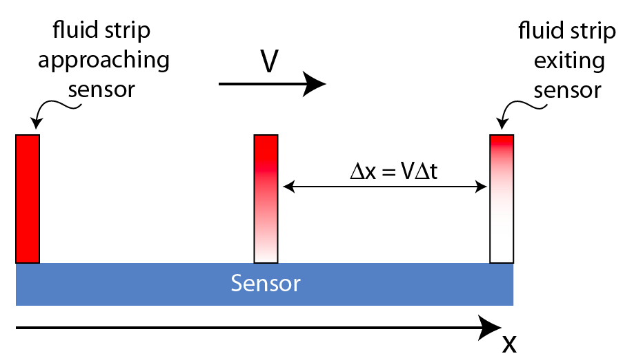
\begin{equation}
t = \frac{x}{v_\infty}
\end{equation}
Where x is the dimension along the sensor direction of flow, x = 0 is the leading edge of the sensor, and 
\begin{equation}
C(x,y)= C_oerf(\frac{y}{2\sqrt{\frac{Dx}{v_\infty}}})
\end{equation}
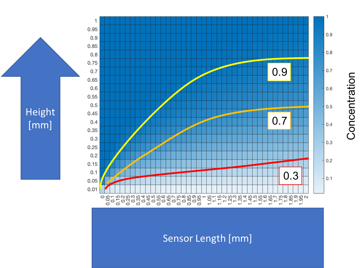
Importantly, the local flux to the sensor is also time invariant …
\begin{equation}
J_o = (D\frac{\partial C}{\partial y})|_o = \frac{D C_o}{\sqrt {\frac{\pi D x}{v_\infty}}}
\end{equation}
Integrating the flux over the sensor length L (and assuming a square sensor) and over time gives a linear relationship …
\begin{equation}
M(t) = 2 C_o L\sqrt{\frac{D L v_\infty}{\pi}} t
\end{equation}
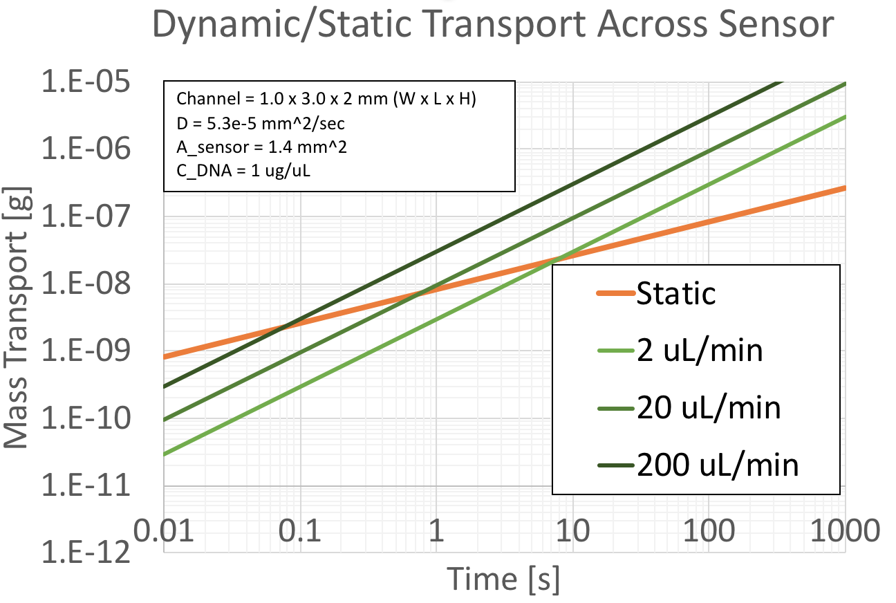
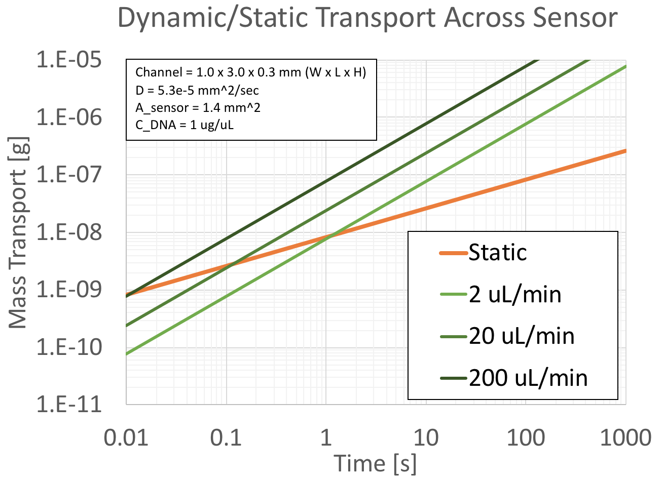

As we reduce the channel height while keeping the volumetric flow rate, the velocity in the channel increases. This improves our transport considerably. Our ‘crossover point’ thereby decreases from 10 seconds down to 0.01 second for reasonable flow rates in our system.