Latest Computer Model of Sieving Looks Terrific
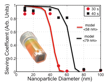
While the membranes cut-offs correlate with the relative pore sizes of the two NPN membranes, neither the average pore sizes (58 nm for 30 s RIE; 79 nm for 40 s RIE), nor the maximum pore sizes (100 nm for 30 s RIE; 120 nm for 40 s RIE) are predictive of the actual cut-off. This is expected for gold filtration in deionized water as the electrostatic and electrokinetic interactions between charged nanoparticles and membranes make the effective pore sizes smaller than their physical dimensions.
transmembranePressurePSI = 3; % We assume the pressure is 5.5 PSI = 37921.16 pascals
zetaMembrane = -0.020; %in V
zetaParticle = -0.015;
molarSaltConcentration = 0.001; %In moles of KCl.
particleDiameter = 20 – 50 E-9;
particleRadius = particleDiameter/2;
poreDiameter = 58 (or 79) E-9;
poreRadius = poreDiameter/2;
membraneThickness = 50E-9; %in m
approxNumberOfPoresInSepcon = 400000000; %(number)
porosity = 0.05; %fraction
activeArea = 1.5E-6; % m^3
fluxthroughpore = DaganFlow(poreRadius, membraneThickness, transmembranePressure); % m^3/s
solventSpeed = (fluxthroughpore/(pi*poreRadius^2)); %m/s
iterations = 300; %number
timeOfSeparation = 2E-7/(fluxthroughpore*approxNumberOfPoresInSepcon); %s
The model was run until 200 uL of the sample had passed through the membrane.
Those curves are reassuring on many levels. Hooray!
One less caveat to worry about, the separations for that figure were done by Sarah and I using constant pressure.
Cheers- Josh
Great! Sometimes it really helps to put these things down for awhile and take a fresh look later.
Can you thicken the membrane and see the curves flatten out in the simulation?