COMSOL simulation on sampling method to measure membrane permeability

Background

We at Michigan have been aiming to perform sequential small volume sampling coupled with our ultrasensitive digital immunoassay to provide longitudinal data from the uSIM. We have encountered repeatability problems as well as low molecule abundancy with shortly incubated samples collected from the bottom microfluidic channel. Therefore, COMSOL simulation work has been done to simulate the secretion of analytes from cells at the membrane to identify the analyte concentration distribution within the 10ul bottom microfluidic chamber in the uSIM. We observed spatial nonuniformity of the analyte concentration which explains the variability as any small fluidic disruption during the manual sampling process is going to largely affect the sampled concentrations. Furthermore, the 2ul sampling at the ports does not sensitively capture the microenvironment concentration close to the membrane area. Therefore, we acknowledged the need of an effective mixing prior to the small volume sampling, or a larger sampling volume is needed to produce repeatable and distinguishable results to target cell secretion behavior towards the luminal compartment.

Extensive work on confocal microscopy imaging to characterize membrane permeability of the uSIM has been conducted at Rochester. Alternatively, Molly recently presents a simple microfluidic sampling method of the complete bottom chamber of the uSIM to perform this characterization without the use of a confocal microscope. The method is comprised of introducing a reservoir to one of the ports and slowly extracting with a handheld pipette on the other port to smoothly sample out the total bottom chamber volume without disrupting the concentration gradient (between luminal and abluminal) and membrane integrity. With the foundation of our previous simulation results, we were able to modify the model to simulate and validate the method is sufficiently exhausting the analyte in the bottom microfluidic channel, thus providing an accurate characterization of the membrane permeability with a given incubation time.

Experiments, Results and Discussions

Two types of boundary conditions were simulated based on the different experimental settings.

i. coated uSIM with cells A constant regulated flux of the analyte across the membrane area is assumed and was found to fit better to the confocal experimental data based on Jim’s previous posts. We therefore back calculated the constant molecular flux based on Molly’s endpoint Lucifer yellow permeability experiments with cells (1hr incubation/diffusion prior to sampling) and input it as a boundary condition in our constant flux model. The diffusion coefficient of Lucifer yellow was taken from a literature and set as 5*10^-10m^2/s. [1] The simulated time-dependent concentration diffusion profile during the incubation is shown below. (Fig.1) With the microfluidic dimensions of the bottom channel, we can safely assume the flow to be laminar. Based on Molly’s experimental settings we introduced a 50ul laminar inflow over a 4s period post incubation to simulate the sampling process. The animation in Fig 1. also shows the concentration profile during the sampling.

Fig. 1. Constant flux 1hr and 50ul extraction of analyte

With the derived values from the simulation, we can plot out the analyte concentration(mol/m^3) at the port surface area at the timepoint of interest. (Fig. 3, Blue lines) This surface average of the volumetric concentration at the outlet port clearly demonstrates sampling at the initial and later phase of the extraction are less sensitive to characterizing the total molecules released to the bottom chamber.  We also output the sampling efficiency (sampled molecules normalized to total molecules released to the bottom chamber after 1hr) with respect to the volume sampled. (right plot in Fig. 3. Blue lines)

ii. coated control uSIM without cells

Without the cell membranes as a regulatory layer, the coated silicon nitride membrane should act as a passive diffusive barrier. Analyte flux across the membrane is modeled using Fick’s first and second law of diffusion where the effective diffusion coefficient is used at the membrane domain and ordinary diffusion coefficient of Lucifer yellow is used at all other fluidic domains. Additionally, we used thin diffusion barrier boundary condition at the membrane to bypass the need of meshing the ~100nm membrane which would cause computational difficulties and errors. The flux across the membrane is determined using the following formula.

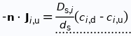
Where D is the effective diffusion coefficient of the membrane, d is the thickness of the membrane and c the analyte concentrations on the two sides of the membrane. The term D/d can be perceived as the mass transport coefficient which is the reciprocal of contact resistance. The initial conditions are a known concentration(150ug/ml in Molly’s experiments) in the luminal compartment (100ul) and an initial 0ug/ml in the abluminal compartment(bottom channel). The effective diffusion coefficient of Lucifer yellow across the silicon nitride membrane were measured and calculated from a previous confocal experiment. The concentration profile after 1hr of diffusion and 50ul of sampling is shown in Fig. 2. and the derived values of concentration at the port and sampling efficiency is compared side to side to the uSIM with cells in Fig. 3. (Orange lines)

 

Fig. 2. Effective diffusion 1hr and 50ul extraction of analyte

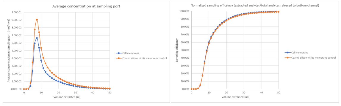
Fig. 3. Sampling efficiency and concentration at port versus sampling volume

Conclusion

Although the overall flux in the coated control is larger than the uSIM with cells, the sampling efficiency-sampling volume relationship is similar to the previous constant flux model. The sampling efficiencies both reach 90% at ~20ul of extraction which demonstrates the 50ul extraction is sufficient to exhaust the bottom chamber analytes regardless of the flux in our range of study. From the simulation results, a total of ~7.99*10^-10 mol of Lucifer yellow is diffused to the bottom chamber which is very close to what Molly sampled out and measured in her experiments.(8.39*10^-10 mol) The difference is a mere 4.8% between the two, indicating our simulation should be valid to represent real experimental scenarios.

References

[1] Micromachines 2019, 10, 533; doi:10.3390/mi10080533