Crazy Colorful Counting Conundrum: From Counts to Colocalization
Summary
We look at nanoparticle counting and colocalization after an ALine device membrane capture and compare IMARIS and ImageJ methods with an example.
Procedures for particle counting and colocalization for IMARIS are discussed and a walkthrough is provided
An example of the observed difference between ImageJ and IMARIS on the observed counts showing a near match on all fronts and an example on the importance to optimize the counting parameters such as the size of the particles and the quality minimum threshold for the best possible counting algorithm.
Introduction
In this post we examine the particle counting problem using a nano-porous membrane and polystyrene beads. Understanding the relationship between capture rate and concentration will be a useful tool when looking further into EV capture. In previous work, the most commonly used software for particle counting has been with ImageJ. ImageJ has tools for examining features and calculating image parameters (mean, median, mode, etc), distinguishing different regions in an image through segmentation, as well as particle counting. One of the frustrating things about ImageJ is that it sees a large conglomeration of nano-particles (NPs) as one particle, leading to severe undercounting. Another problem is the subjectivity of the program, with the thresholds that it uses to distinguish a particle from another particle, by the intensity profile and size. One of the major benefits of ImageJ however is that it is free to use. Another software package that has been used to count NPs is IMARIS. IMARIS has many of the same features as ImageJ, but with a much more user friendly user interface. ImageJ and IMARIS do not differ by a lot when looking at the way that they count particles, still using particle size and an intensity threshold, however IMARIS can count particles in 3 dimensions using a Z-stack. IMARIS is an expensive tool, but with the right license can perform analysis on an entire folder of images in a short period of time. In this post we look at how to use IMARIS to count particles, and as a way to incorporate the EV counting project, we look at performing colocalization on an image with more than two channels.
Methods
Particle Counting
In order to start the particle counting process, understanding the IMARIS interface and file structure is important. Below, you see the file structure for the concentration ladder that was used to compare IMARIS to ImageJ. Each small folder has three images in it that are triplicates of the same ALine device in different locations to try to minimize error from one image.
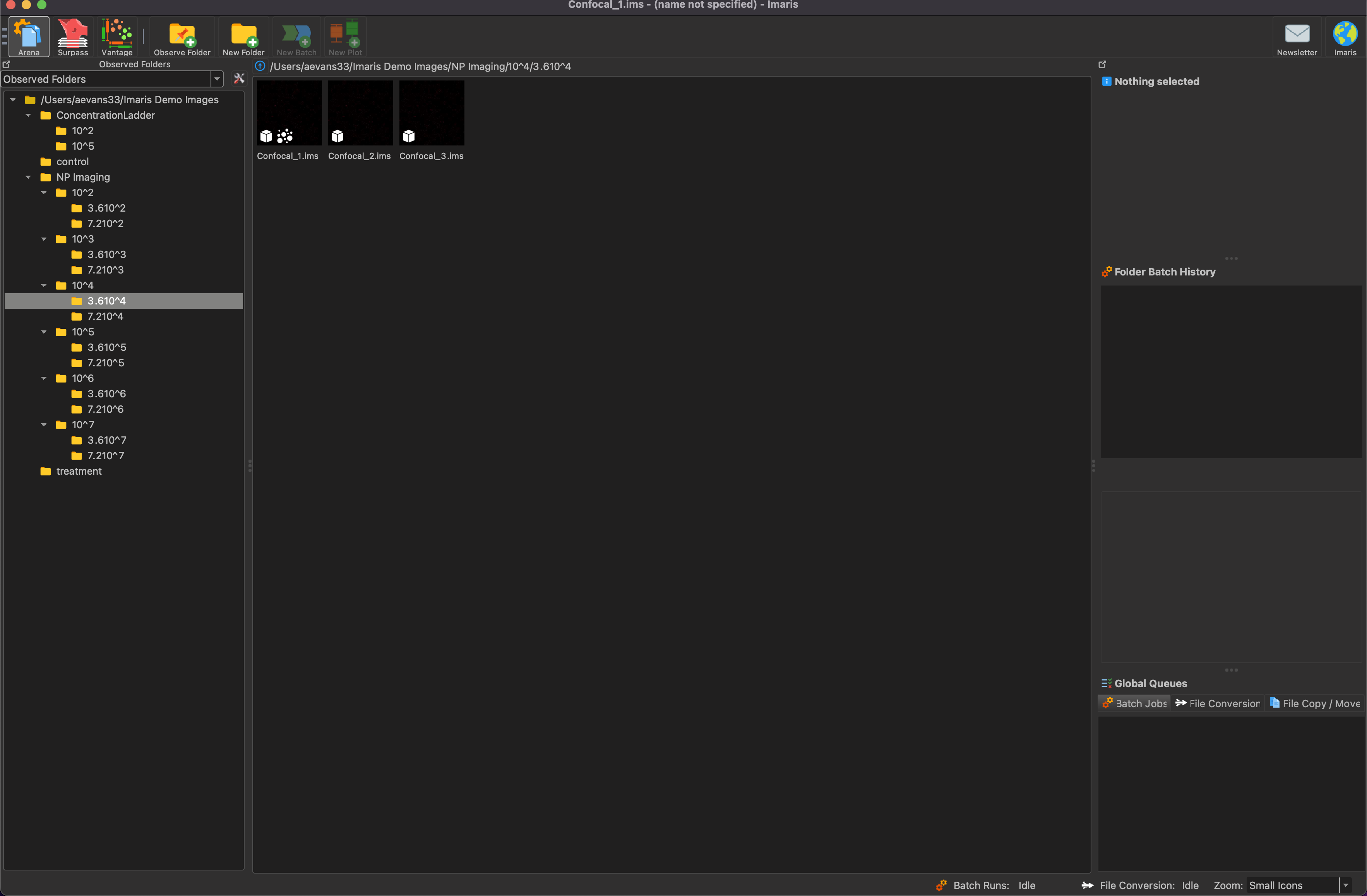
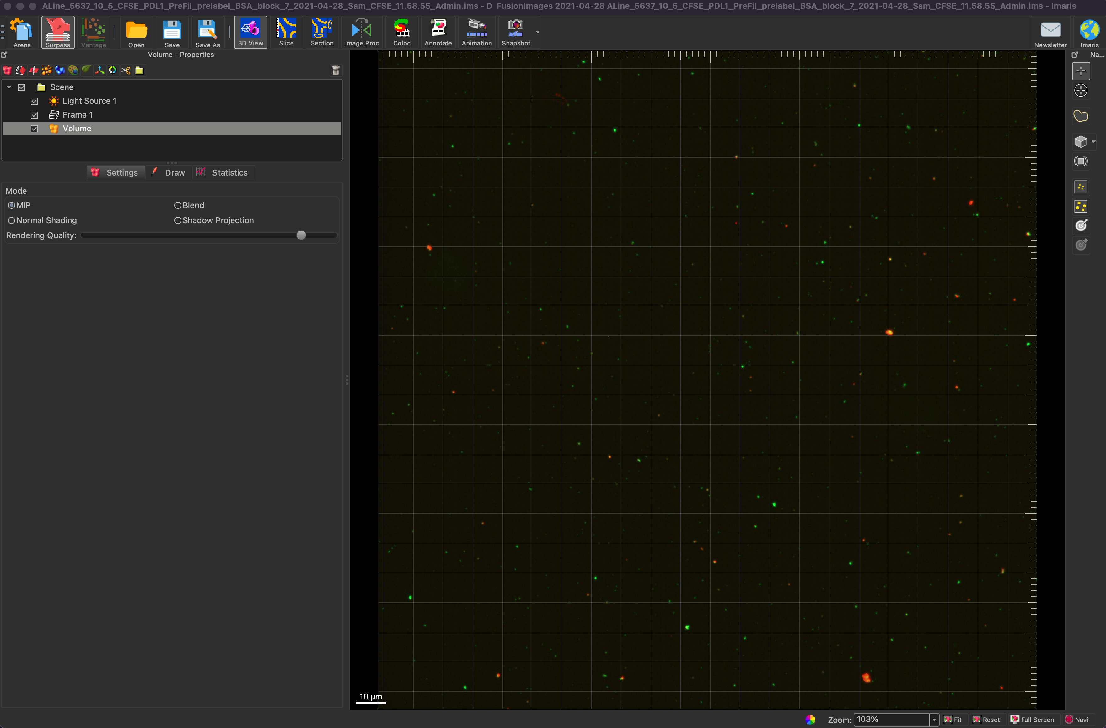
Double click on the image that you want to process and it will open up like the image shown below.

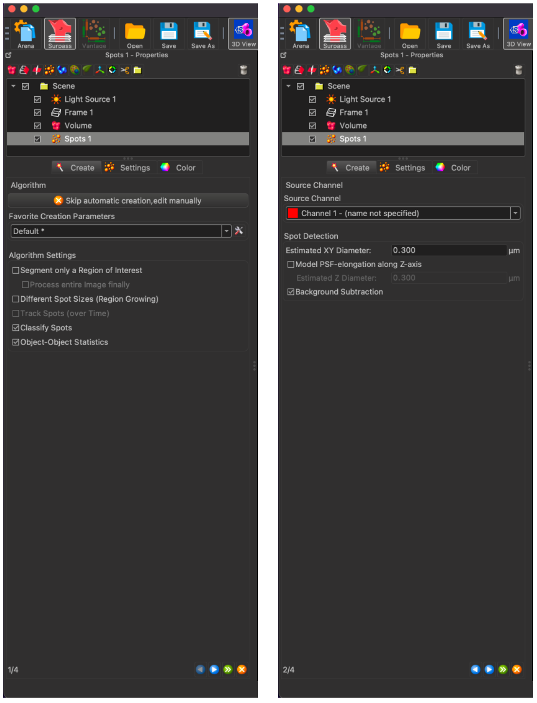
To create spots on an image, click on the spots icon in the top right of the image (The one that has yellow-orange bubbles) and the below spot creation interface will open. There is no need to change any of the settings on the first page, but the second page allows for the channel selection and the estimated diameter of the particle that you want to analyze. If you get a low count on your image, increase the particle diameter until you see IMARIS count hundreds of thousands of particles. This number does not affect your results, but if you capture all of those spots, the spots will cover the entire image.
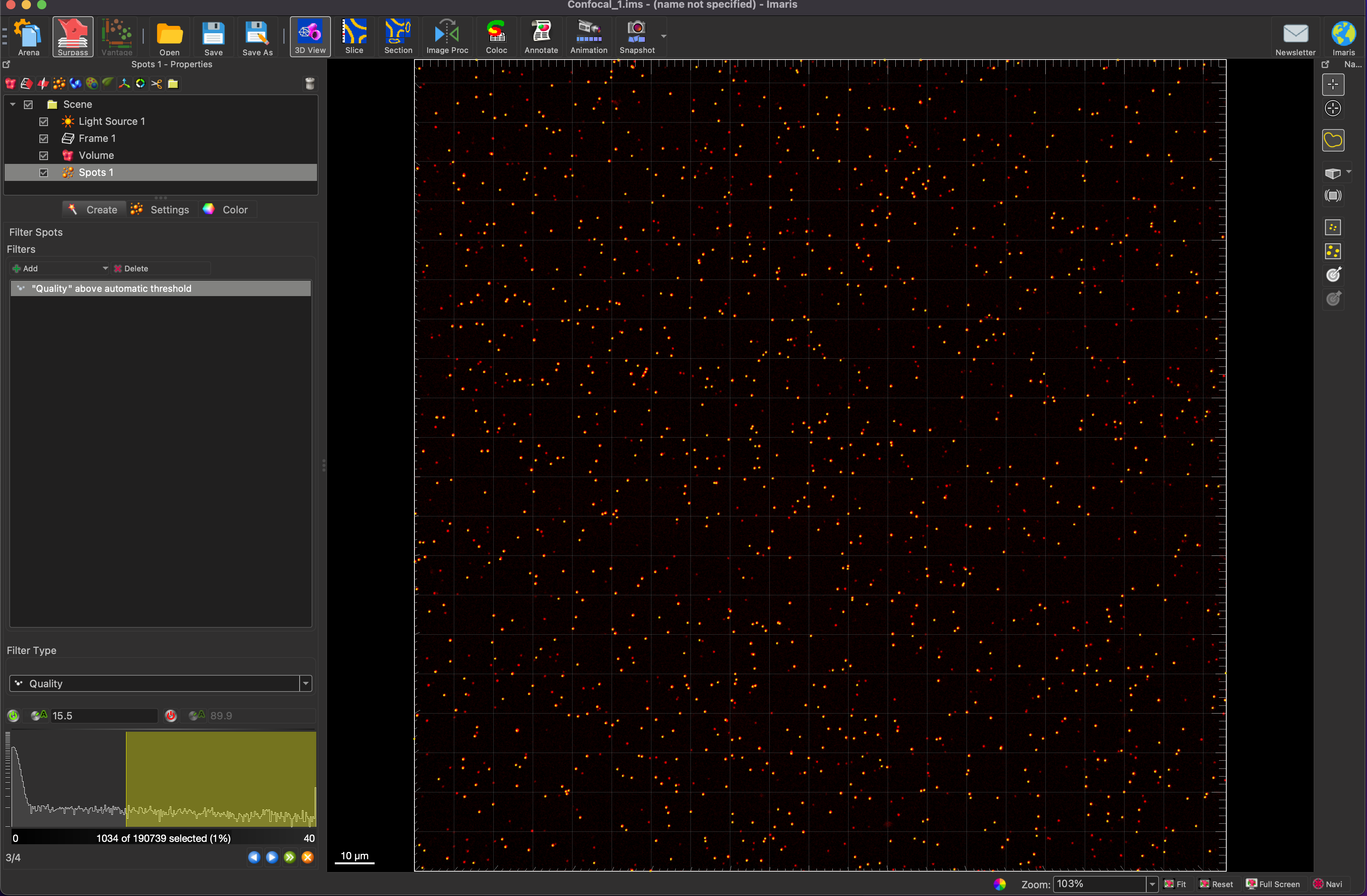
In the below image, you can see the automatically calculated threshold generated by IMARIS. This threshold can be adjusted as seen in the second image below. In this case, the quality threshold was set to 5.00

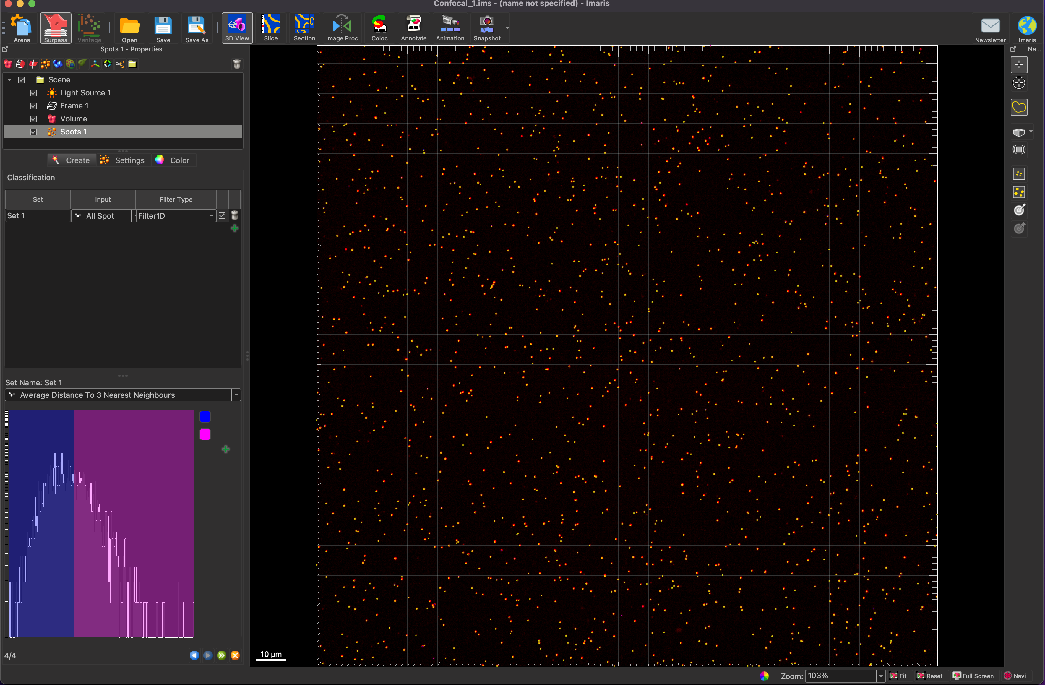
The final step of the spot generation allows for you to classify the spots into different groups. This feature was not explored in the scope of this rotation, but it allows you to separate spots by size, area, position, and a number of other classifiers. This can also be ignored for now and done later in a filter (will be shown later).
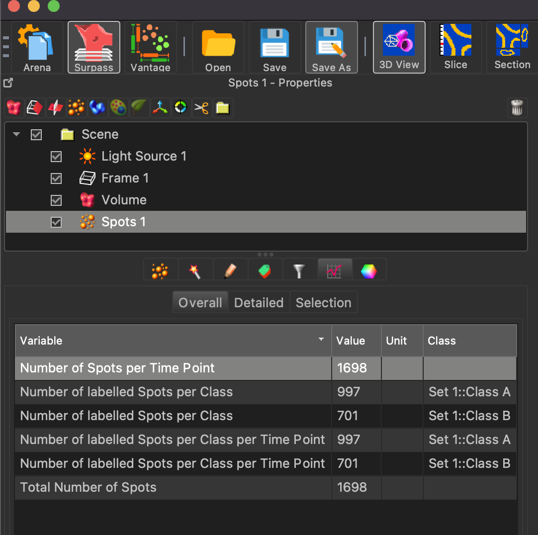
After the spot generation is completed, click on the statistics tab under the spots feature, and you will get a spot count that can be recorded for image analysis.
Colocalization
To determine show colocalization between two channels, we first choose an image with two or more channels. Below we see an image with green EVs and red antibodies.
First we create two different spots, one for each channel. Below they have been named green and red, and in this image the spots were given a radius of 0.600 um. This number is important for choosing the interaction length for later steps. In this scenario a quality of 2 was chosen to separate spots from background.


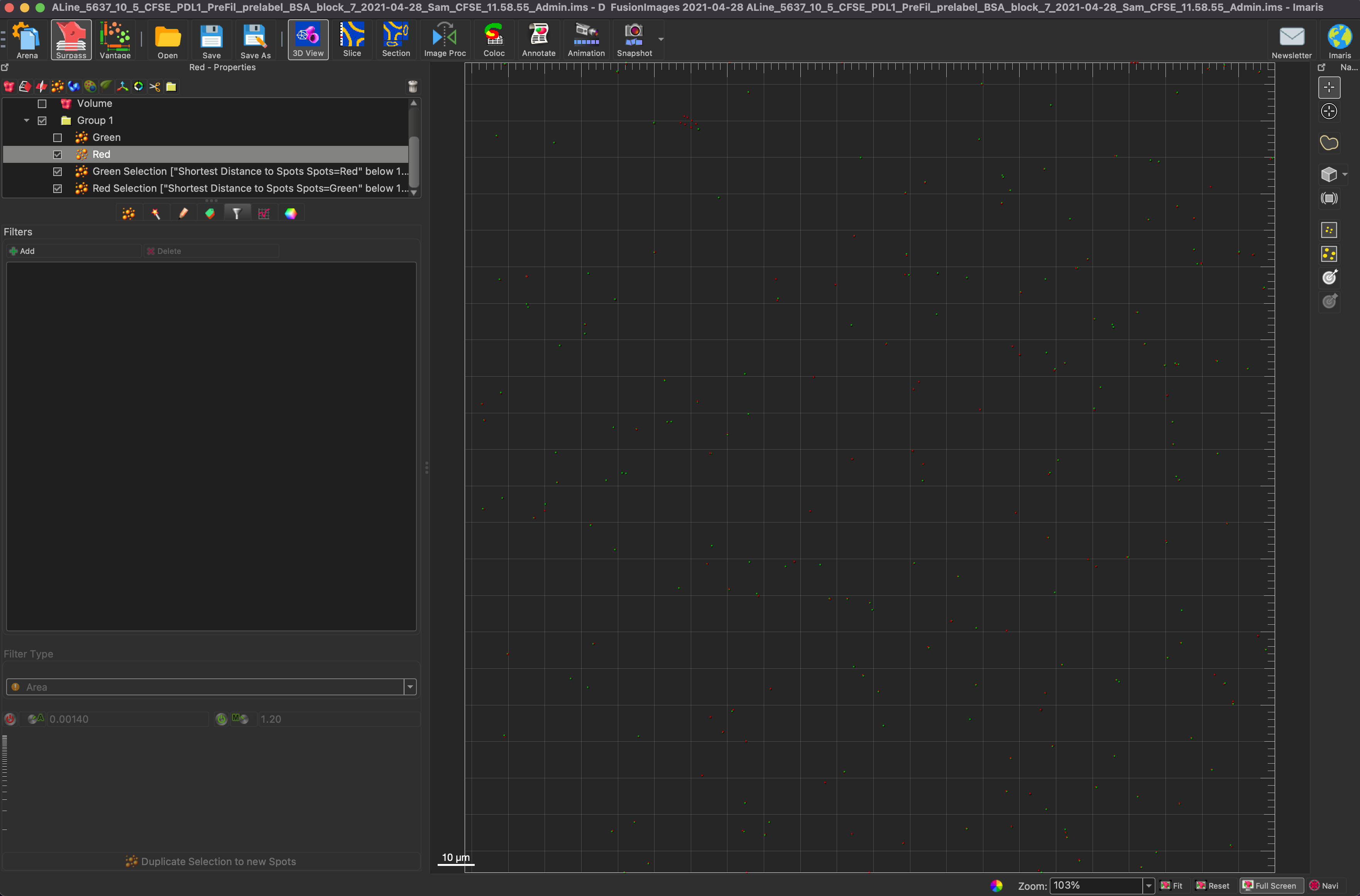
Now to perform the actual colocalization part. First select the green spots and click on the filter tab under the green spots. Choose the “Shortest Distance to Spots Spots=Red below 1.20” filter, which translated to find green spots that have red spots within 1.20 um of them and select those green spots. Repeat the same steps for Red. The reason for the 1.20 um is the two radii added together, so if the particles are touching, there is colocalization. IMARIS also takes the Z position of a particle into account when performing the above calculation, unlike ImageJ which has to do it on a 2D image.


To better visualize the spots, you can turn off the background image after the spots have been generated. This shows only the colocalized spots rather than the whole sets of spots. The first image below shows only the colocalized spots, while the second image shows all of the spots, and the third image shows the green colocalized spots and all of the red spots. This better shows the difference between the two sets of all spots and just the colocalized spots.


To get all of the necessary statistics, you must put all of the groupings of spots into a group. To add a group, click on the folder above the image properties. Click on the statistics tab while the group is selected, and the counts of green spots, red spots, colocalized green spots, and colocalized red spots will be available. In order to calculate the percent colocalization, the count of colocalized red spots must be divided by the count of all green spots. In order to find the colocalization efficiency, take the colocalized red spots again, and divide it by the total number of red spots.

Both of the above methods allow for particle counting and colocalization. If a batch processing feature is added to the IMARIS License that will allow these parameters to be set for all of the images in a folder, meaning that IMARIS can potentially run all of these analyses in one go and output all of the results in an excel spreadsheet.
Results
In order to visualize the comparison between the counting algorithms of ImageJ and IMARIS, a concentration ladder of polystyrene beads was created that had bead counts of 3.6*10^2 up to 7.2*10^7. The parameters used in IMARIS had a quality of 5.00 and a radius of 0.600 um. Each set of beads had 3 separate images and the counts of those images were averaged and then multiplied by 33.05, which is the total number of fields of view, which gives us an approximate capture count. Those capture counts were compared to the actual number of beads in the device based on dilutions of the stock solution. The following graph shows the comparison between IMARIS and ImageJ.
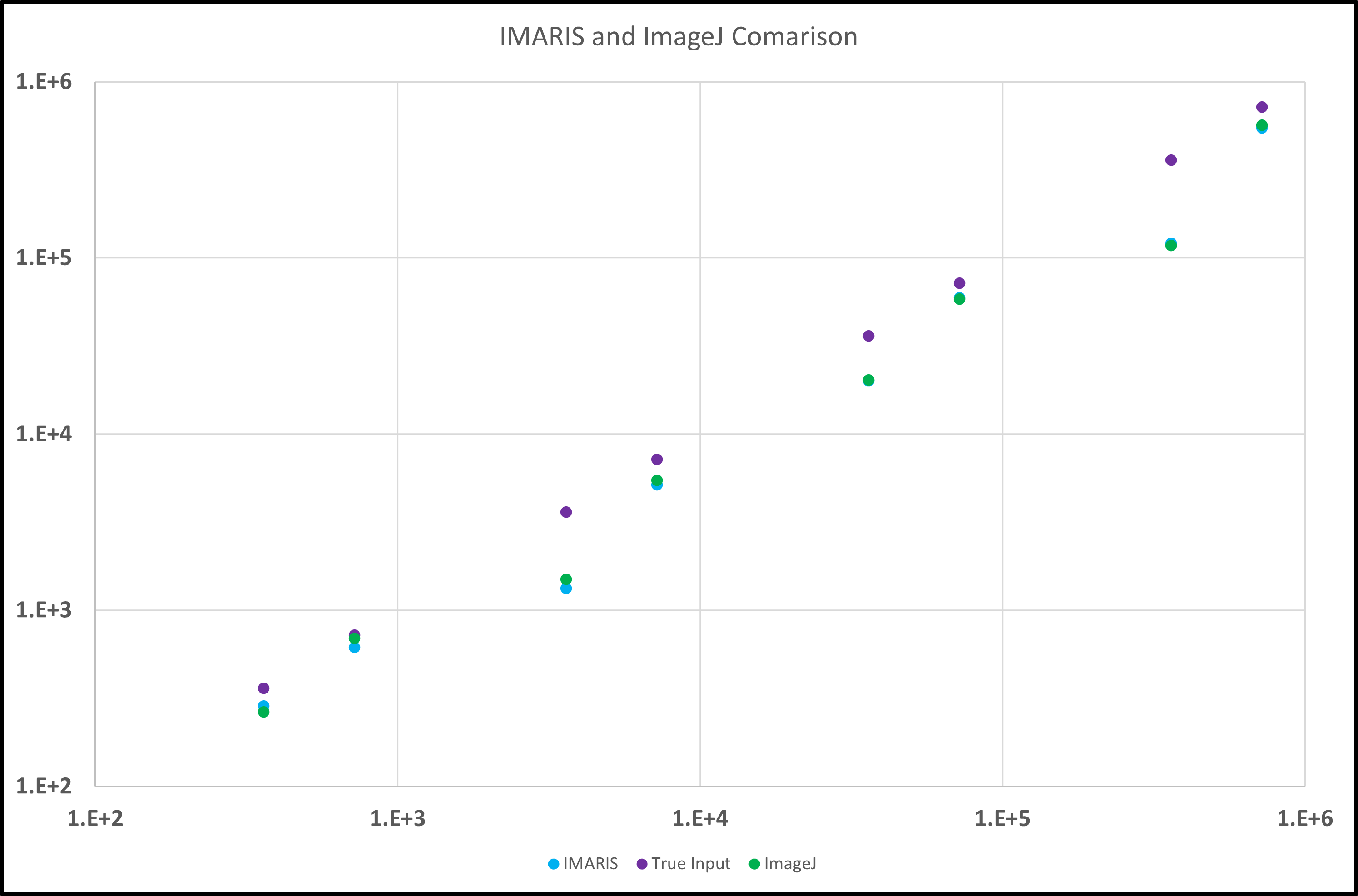
As seen in the above graph, the IMARIS and ImageJ counts are very close to each other in all of the images analyzed. In order to improve these counts to get closer values to the actual amount, the quality parameter may need to be adjusted and optimized for each of the analyzed images into a more accurate “one-size-fits-best” solution. Evidence for this is highlighted in the below chart.
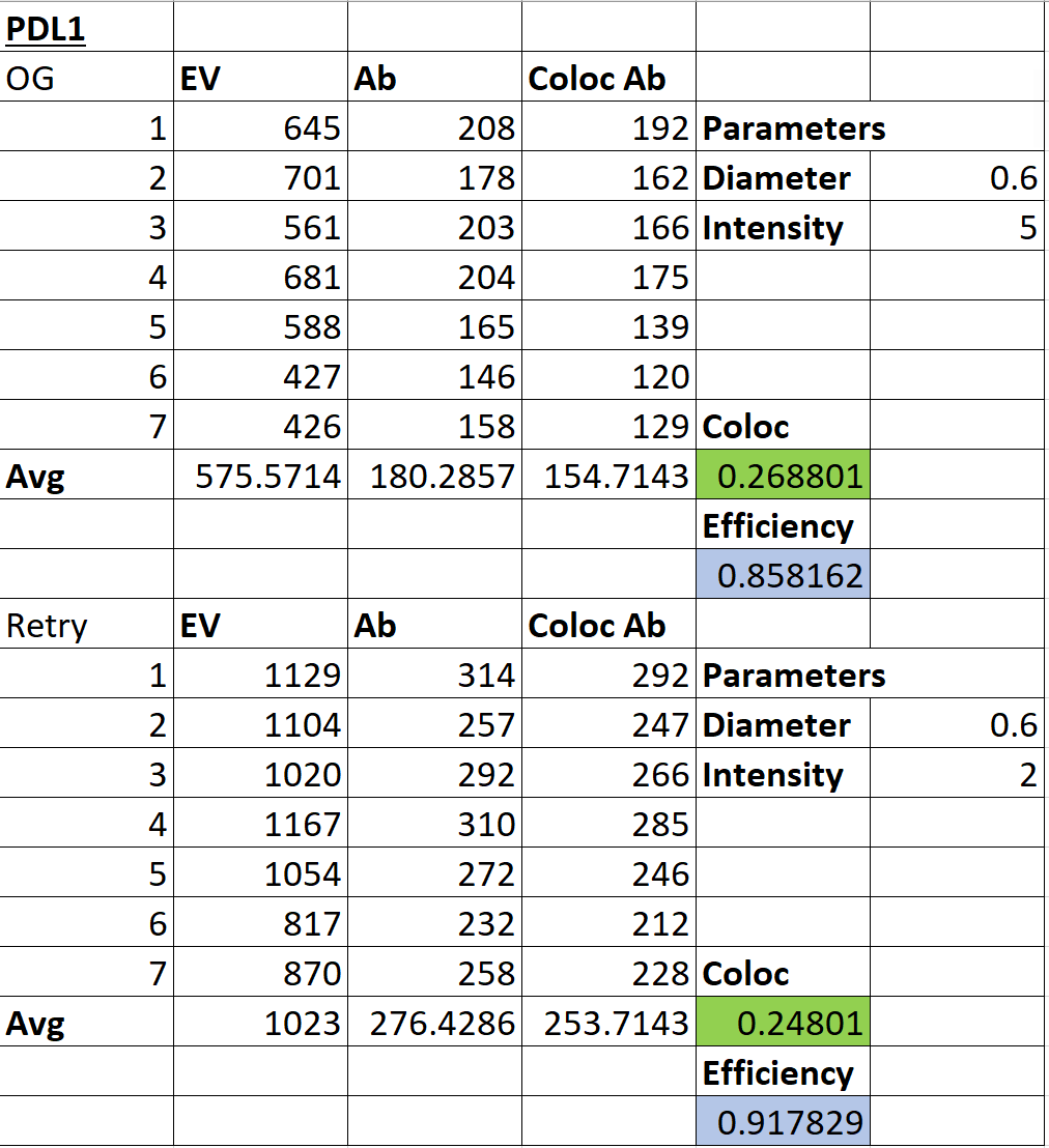
When the quality parameter was changed from 5 to 2 in the above table, the counts for both the EVs and the antibodies increased by a significant amount, and these counts better matched the previously recorded ImageJ counts. This just provides evidence that optimization is necessary to have a better algorithm for particle counting.
Conclusion
In this blog post, methods for particle counting and colocalization in IMARIS have been discussed as well as the need for an optimized set of parameters in the particle counting problem to best match the expected data. The error between the expected and observed data for the particle counting is very similar between IMARIS and ImageJ for that set of parameters, but adjusting the IMARIS parameters may result in better counts, matching the expected model better than the original parameters.
Sources
https://imaris.oxinst.com/packages
https://www.youtube.com/watch?v=1UmBawtqQbE&t=134s