Modeling Diffusion with COMSOL
Due to the discrepancies between the 1D model and experimental runs with rhodamine, I have switched over to using COMSOL to solve for a 3D model. In this system, 200×200 um membrane squares with a 45 degree etch separate the two wells. The top well is set up with .5 mol/m3 of rhodamine, and the bottom has none. The diffusion coefficients in the model are set at free diffusion, except for the 15nm membrane slice, which has an effective diffusion coefficient. The system is meshed (using a swept mesh for the ultrathin membrane segment) and solved for a 24 hour period.
To determine the effective diffusion coefficient, I’ve used the principles of my previous model. In essence, I’ve added the resistances due to steric hindrance and finding a pore in series and calculated a diffusion coefficient from the total resistance.
Results:
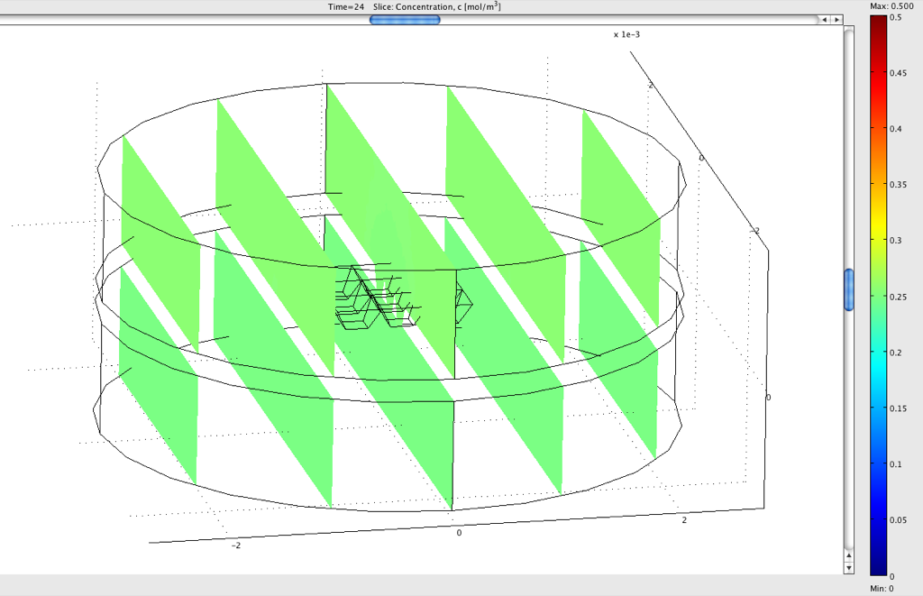
1x well chip
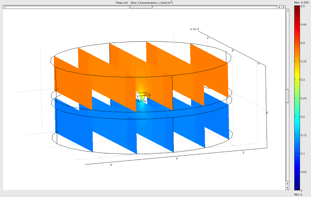
While diffusion has occurred, this chip is not at equilibrium in 24 hours. The ratio of filtrate concentration to retentate concentration in this simulation is 0.33.
3x well chip
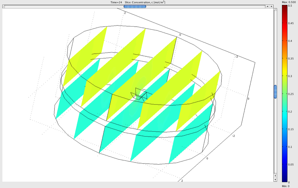
This one is a little further on. Ratio is 0.71.
6x well chip
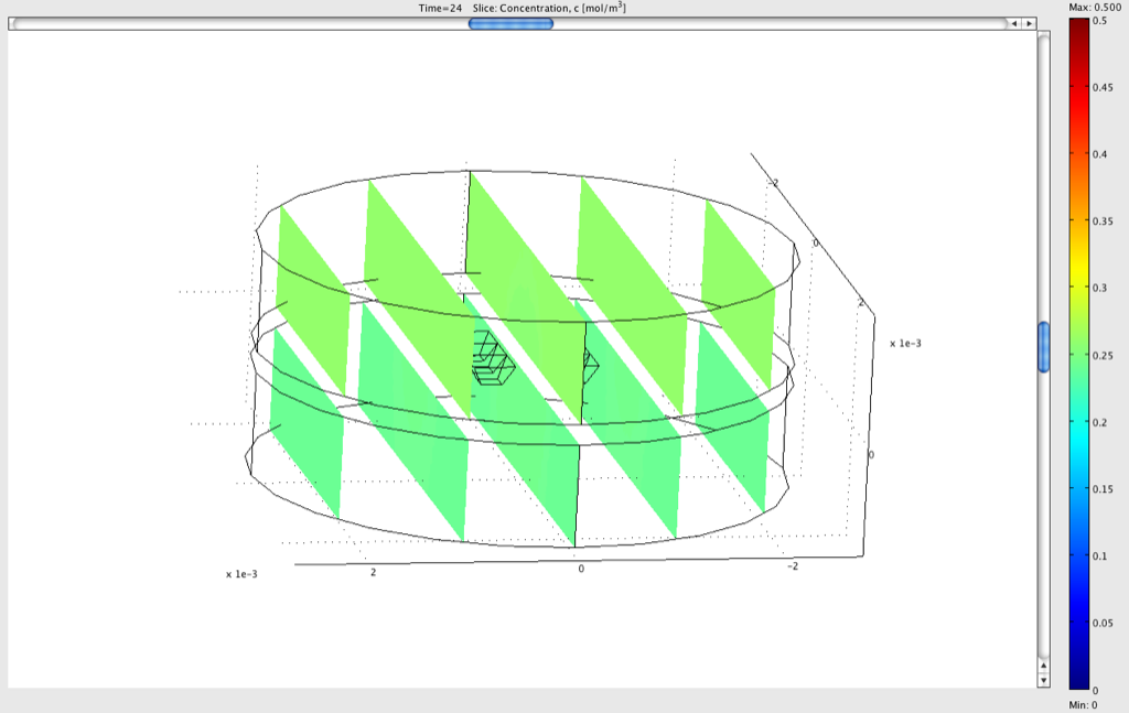
Close to equilibrium. Ratio is 0.92.
9x well chip
This system is almost at equilibrium. Ratio is 0.96.
I recently finished the rhodamine diffusion experiments for all geometries. Here are the results in terms of ratios after 24 hours:
| # of squares | experimental ratio | COMSOL ratio |
| 1 | .23 | .33 |
| 3 | .60 | .71 |
| 6 | .83 | .92 |
| 9 | .90 | .96 |
So we’re not quite on, but this is a lot better than previous attempts. Next I will be working on plotting ratios over time and working up to steric hindrance with large molecules.
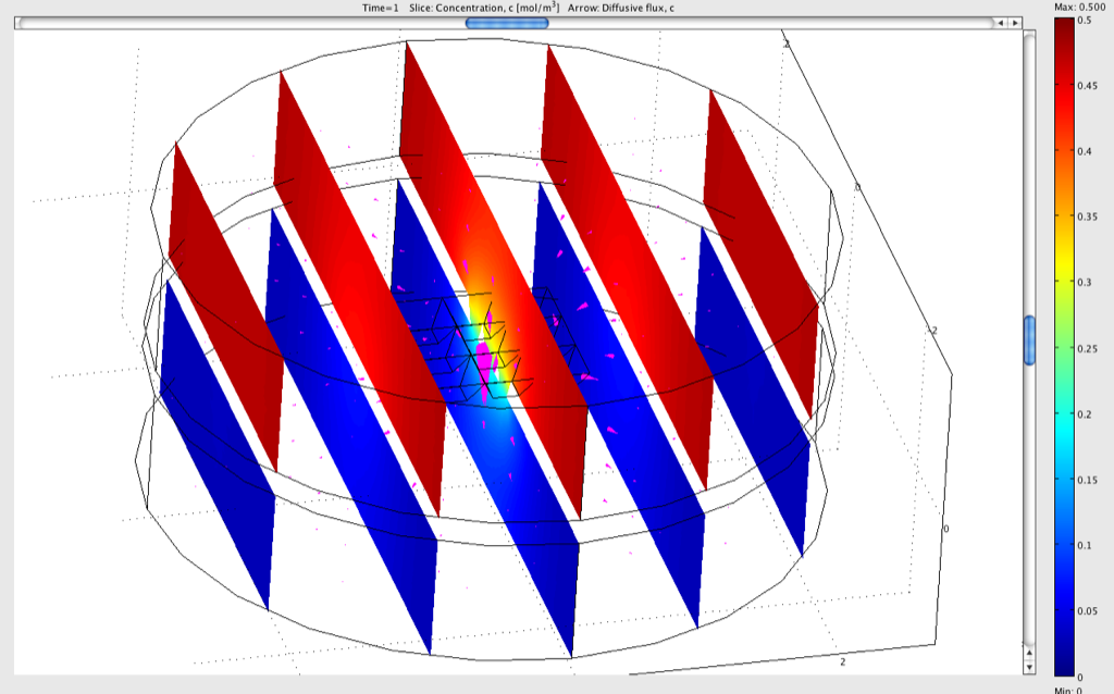
P.S. Cool picture- 9x squares after 1 hour with pink arrows indicating diffusive flux: