Microfluidic Permeability Assay for In Situ Monitoring of Endothelial Barrier Properties

Introduction

As part of my thesis, I have been working on developing an assay for measuring vascular barrier properties within our microfluidic devices. Traditionally, small molecule permeability measurements are performed on cells plated in a Transwell cup. The basic protocol for these assays is initiated by introducing FITC-dextran in cell culture media into the apical compartment of the device. After waiting a discrete amount of time (depending on assay conditions, personal preference, detection limits, etc.), media is collected from the basal compartment and transferred to a 96-well plate. These plates are placed in a fluorescence reader and analyzed for basal FITC-dextran concentration. This concentration can be inputted into the following equation (1) to obtain endothelial monolayer permeability:

Were Pe represents monolayer permeability, J is change in concentration over assay time, A is membrane area, and C_o is the FITC-dextran concentration added to the apical well.

While this assay may be suitable in the Transwell format, the small reservoir volumes in our microfluidic devices make it extremely challenging, as sample collection may itself disturb the monolayer integrity. This main concern sparked our interest in developing a novel protocol for monitoring small molecule permeability within our devices. Furthermore, we hope to make this assay facile, without the need for specialized equipment as necessary for previously developed transendothelial electrical resistance (TEER) systems.

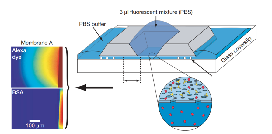
In the early days of silicon membrane development in our lab, Striemer et al., demonstrated a protocol in which transport of fluorophore through a nanoporous membrane was monitored via an epifluorescence microscope. This assay was utilized to show how fluorescent BSA is held back by the nanoporous membrane, while Alexa dye freely diffuses through (Figure 1). Inspired by this protocol, we hypothesize that transport of FITC-dextran through the endothelial cell layer and nanoporous membrane, into the basal channel of our microfluidic device, can be monitored with an epifluorescence scope, and would be predictive of endothelial cell layer permeability.

Materials and Methods

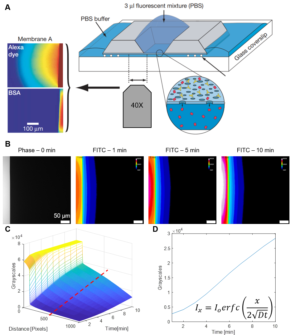
For reference, all experiments herein were performed in and model after the Aline devices [See post here]. After cell culture and desired experimental treatment, devices were be prepped as follows: Microfluidic devices were rinsed thoroughly with cell culture media. The apical and basal chambers were be loaded with fresh, warm (37 C) media and the device was placed on a fluorescent microscope stage. A 40X objective was focused directly under the nanoporous membrane, with a majority of the view blocked by the silicon scaffolding surrounding the freestanding membrane (Figure 2A). For field of view reference, a phase image was taken (Figure 2B). Media was removed from the apical chamber and replaced with a 2 ug/ml solution of 40 kDa FITC-dextran [Sigma] in cell culture media. Fluorescent images were recorded (Ex/Em 495/519) once a minute for ten minutes with a short exposure (200 ms) to minimize photo-bleaching (Figure 2B). After the experiment, the working 2 ug/ml FITC-dextran solution was passively pumped into the bottom channel of the device and a final image was taken (necessity explained in forthcoming section; video at end of post). The images as described above were then imported into a custom made Matlab script, within which the pixel intensities (grayscales) are averaged down the y-axis, and plotted on a 3D mesh over time (Figure 2C). The pixel intensity 50 μm from the freestanding membrane edge is extracted from the data set and plotted over time (Figure 2D). In this form, we may now speculate on how we can obtain a measure for endothelial monolayer permeability.

Defining Diffusion Through a Single Point Over Time

In the course of this work, Jim and I wanted to find an equation that defined the flux of FITC-dextran through our cell layer over the time of the assay. Our first instinct was to use equation (1) as shown above, as this have been used in the past for small molecule permeability measurements, and made the most sense. Quickly, however, we realized that this equation is not suitable for our work, as it requires the ability to measure the concentration of the small molecule that passes through the membrane into the basal channel, and we are merely observing a small subsection of the system. Therefore, we scanned a textbook on diffusion [The Mathematics of Diffusion by J. Crank] for a solution to Fick’s Laws with the proper boundary conditions that most closely mimicked our experimental configuration. In so doing we found the following equation (2):

 

Where C_x is the concentration of the small molecule distance, x, from the source. C_o is the source concentration, D is the diffusion coefficient of the small molecule within the system, and t is time. This equation is derived from Fick’s Second Law, and describes diffusion through a semi-infinite medium with a constant source. The boundary conditions are as follows:

By consulting Beer-Lambert law, relating small molecule concentration to absorbance (and therefore fluorescence in some cases), we can put equation (2) into the following form [equation (3)]:

Where I_x is the fluorescence intensity given off by the small molecule distance, x, from the membrane source, and I_o is the fluorescence intensity of the working solution (that was loaded into the apical chamber). Interestingly, if we divide I_o through the equation, the left side becomes unit-less (a ratio of I at point x to I_o). Experimentally, we can extract this exact variable over time, effectively allowing us to fit equation (3), and obtain a value for D. More specifically, the graph in Figure 2D represents I_x, when x=50 μm, and the portion of the experiment where the working solution is passively pumped into the basal chamber gives us a value for I_o. When I_o is divided through the data, we can fit the trend to some value of D.

With a value for D, we now need a way to obtain a value for endothelial cell monolayer permeability as traditionally done in literature. Permeability of a system is defined by the diffusion coefficient within the system over the travel distance (D/L). To this end, we can predict the permeability of the microfluidic system (cells + membrane + bottom channel) is equal to the value for D obtained above divided by L (50 µm). Next, we can use equation (4), to obtain a value for monolayer permeability.

Were P_total is the permeability of the system (D/L from experiment), P_EC is the permeability of the monolayer, P_NPN is the permeability of the membrane, and L/D (far right) is the length from the source to the detector (50 µm) divided by the native diffusion coefficient of the 40kDa FITC-dextran in 37 C media.

Using COMSOL to Predict Experimental Outcomes

While a lot of analytical solutions are laid out above, they do not directly reflect the experimental setup. With this apparent shortcoming in mind, Kilean and I sought to replicate the experimental configuration in the FEM software, COMSOL. In brief, we modeled the diffusion of a species (with diffusive properties identical to that of 40 kDa FITC-dextran) through a 2D slice of our microfluidic device (Video 1).

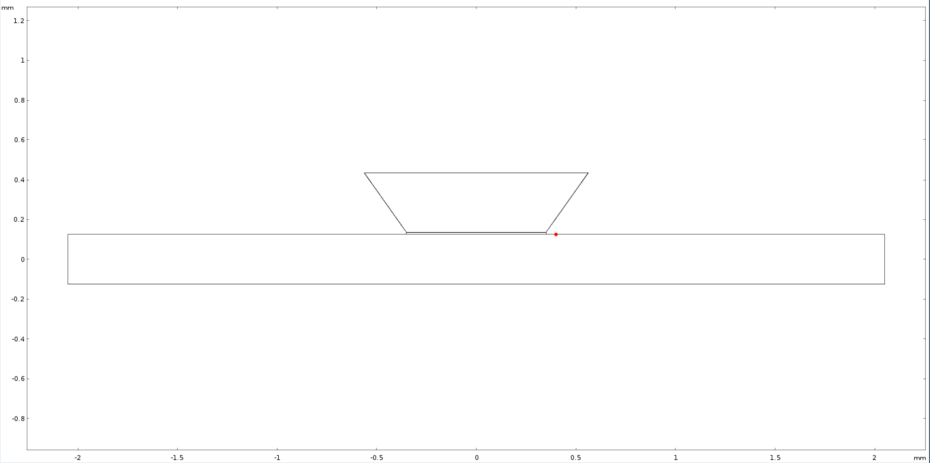
To more closely mimic the experimental setup, concentration changes through a single point 50 μm from the membrane (coordinates 0.4 mm, 0.125 mm; mimicking objective based data collection; Figure 3) were collected from a 10 min simulation (one point for every minute as performed experimentally). This data was plotted along with the solutions for equation (2) within the experimental parameters (Figure 4). After seeing a variation in the FEM data and analytical data, and fit for D (D*) was determined and plotted.

 

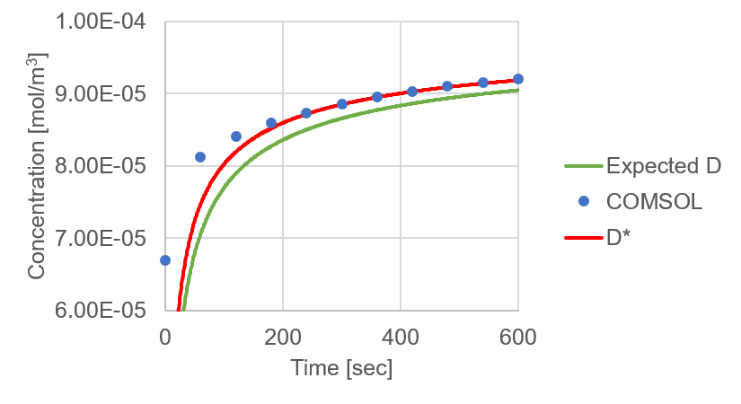
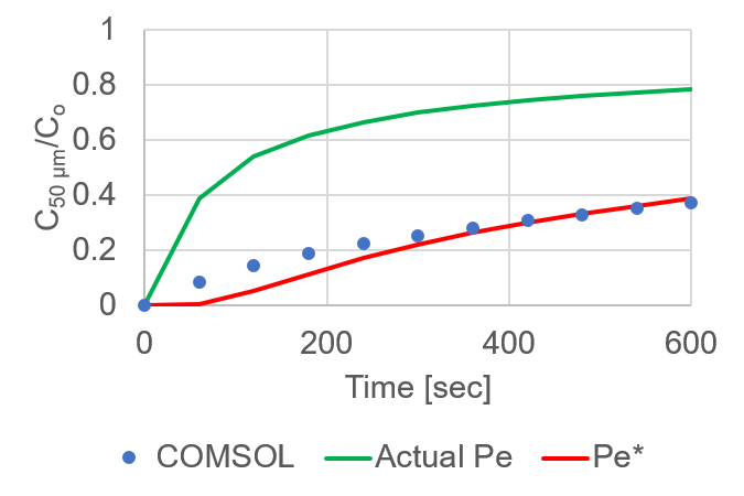
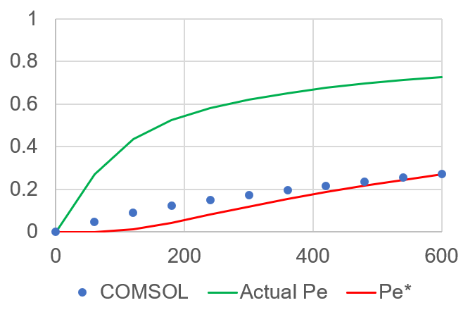
This data shows that while equation (2) is quite predictive of our experimental setup, it is not without a margin of error (difference between D and D*). Due to this error, we decided to slightly alter our experimental approach. As opposed to relying on the analytical fit of our experimental data, we would like to build a large COMSOL data set that modeled a variety of endothelial monolayer permeabilities (within a reasonable range) and would allow us to fit our experimental data to a defined permeability coefficient. To start this, Kilean added a 10 μm tall rectangle between the trench and the basal channel to represent an endothelial cell layer. Videos 2 and 3 show examples of concentration progression when the permeability of the ‘monolayer’ is set to high (Video 2) versus low (Video 3). Since we know permeability is equal to a diffusion coefficient over some distance, we changed the diffusive properties of this rectangle to equal that of a confluent endothelial cell monolayer (permeability data provided by Dr. Glading’s lab at URMC, I input this data into equation (1) to obtain a permeability coefficient, and back calculated a value for D based on the height of the rectangular layer, 10 μm); Pe = 8.88E-5 cm/s, D = 8.88E-12 m^2/s. I again ran the COMSOL simulation, and extracted the time-dependent concentration change through a point 50 μm from the membrane edge (Figure 5). Using equation (4), I back calculated a system diffusion coefficient and input that into equation (2) (Figure 5, Green line). Additionally, I fit the COMSOL data to equation (2) (Figure 5, Red line). As depicted, the COMSOL data did not match the mathematical model. Interestingly, the mathematical calculation for D and the COMSOL fit for D are exactly 1 order of magnitude off (2.78E-12 m^2/s vs 2.78E-11 m^2/s; Mathematical vs COMSOL).

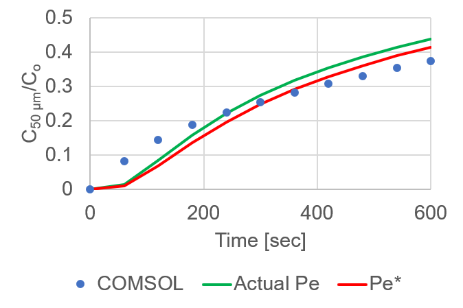
Since this difference seemed too exact to be a model error, I repeated the COMSOL simulation with a new permeability value (4.44E-5 cm/s). Again, the difference between the COMSOL predicted D and the mathematical D are off by 1 order of magnitude (1.71E-12 m^2/s vs 1.71E-11 m^2/s; Math vs COMSOL; Figure 6).

This is where I am stuck. I find it hard to believe that I don’t have a unit error in my solution or COMSOL model, but Kilean and I rechecked our COMSOL model and couldn’t find any error. Something to note, the poor fit of equation (2) at early time points to the COMSOL model seems to be an increasing trend with decreased monolayer permeability. I suspect this is do to variation in the diffusion pattern that is emphasized as the monolayer greater influences the overall system permeability.

Update with Solution (03/28/2019)

After reviewing my COMSOL model again, I decided to run another experiment that more closely followed the rules of the derived equation (2). More specifically, equation (2) is meant to represent diffusion from a central source through a point distance, x, from the source. Our experiment doesn’t quite follow these rules as the point we are looking at is not directly below the source, but instead is off to the right (Figure 3). However, if I were to move that point in COMSOL to a more ideal location, I can more accurately predict if the model is correctly mimicking the mathematics. To do this, I changed my point at which I monitor concentration change to 0 mm, 0 mm (Figure 7). After running the simulation, I plotted the concentration changes with respect to time, and plotted equation (2) with identical parameters (Figure 8). While the fit is not perfect (RMSE = 0.045), it shows great agreement with the mock experimental data, therefore we can conclude the model is correct.

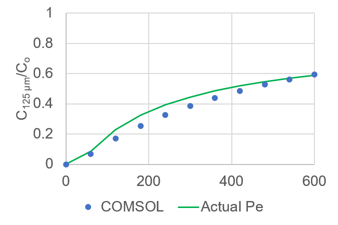
This validation greatly disproved my unit error theory, so I went back into my mathematics to see where I may be going wrong. One variable this new experiment made me more aware of is the distance, L, that is used to convert D* to permeability in equation (4). This would also mean that x in equation (2) would have to change to reflect that new value. After some thought I decided to change these values to represent the distance from the center of the source (membrane) to the detector, equaling 400 μm. When I make these changes, the new data shows much better agreement (RMSE = 0.05; Figure 9, Green line). After iterating through some equation (2) fits for the COMSOL data, I did find a value for permeability that had a slightly lower RMSE (0.044; Figure 9, Red line). I would conclude, however, that this difference is within reason for experimental purposes, especially when considering permeability variation is usually plotted on a log scale.

Conclusion

We have successfully validated our math and COMSOL model, and are ready for experimental data!

Future Work

This work will be featured in a manuscript we would like to submit next month. In order to validate our model further, we will be working in collaboration with Dr. Galding’s lab at URMC to obtain some example permeability data, both in the traditional transwell format as well as using our methods. We hope to develop a protocol to get these two models to agree so we can ensure reliability for future work and collaboration.

Update with Transwell Data (04/08/2019)

Dr. Glading’s lab has provided Transwell permeability data for comparison. I decided that prior to running the in situ permeability assays, we can predict the tolerance of our assay in detecting permeability changes as suggested by the Transwell experiments. Briefly, human pulmonary aortic endothelial cells (HPAECs) were grown to confluency in 12-well transwell inserts. For thrombin groups, 2 U/ml human thrombin was added prior to permeability measurements. Transwells were washed and a working solution of 2 μg/ml 40 kDa FITC-dextran was loaded into the top chamber. Transwells were incubated for 2 h and abluminal media was aspirated. Abluminal FITC-dextran levels were measured in a plate reader and reported in μg/ml. This concentration was converted to J by multiplying the reported value by the bottom well volume (1.5 ml) and dividing the resulting number by the assay time (2 h). J was input into equation (1), and a permeability was calculated (Figure 10).

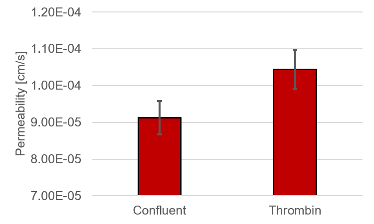
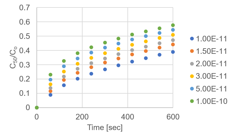
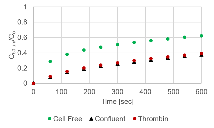
These permeability values were then loaded into the COMSOL model and resulting concentrations at the “detector” were recorded. These data were divided by initial concentration (2 μg/ml) and plotted (Figure 11). Unfortunately, the difference between thrombin treated and confluent HPAECs seems to be too close for our assay. Considering this is supposed to be experimental extremes, this could be problematic. Fortunately, literature usually reports these changes in permeability in order of magnitude differences in permeability, therefore the results reported here are not normal. I am confident that if these values do trend to order of magnitude differences we can predict changes in EC permeability.

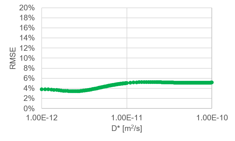
For reference, I ran a parametric sweep of 200 ‘expected’ permeability values, and the RMSE does not rise above 5.5% in any case (Figure 12).