Localizing Basement Membrane Production in Coculture BBB Model
Introduction
The basement membrane (BM) is a critical component of a healthy blood-brain barrier (BBB) model. Further, the BM breaks down in several diseases. Both pericytes and endothelial cells can contribute to basement membrane production. This post will explore a method to localize basement membrane components – collagen type IV (Col IV), fibronectin (FN), and laminin (LM) – in a coculture BBB model in the µSiM.
Cell Culture and Image Acquisition Methods
IMR90-4-derived brain pericyte-like cells (BPLCs) and EECM-BMEC-like cells were cultured in µSiMs, separated by trench-down NPN membranes. Briefly, BPLCs were seeded on the top surface of uncoated channels, and the following day EECM-BMEC-like cells were seeded in ColIV+FN-coated top wells. Cultures were grown for 5 days after EC-seeding and live-stained for basement membrane components.
Confocal images were acquired on the Andor Dragonfly Spinning Disc Confocal using z-stack. The stack includes the top of ECs to the bottom of PCs (including all BM). Step size is set to 0.2 µm. In this post, I acquired with a LWD 40X objective, but 20X may be more optimal. I take 1-3 images/device and plot everything separately.
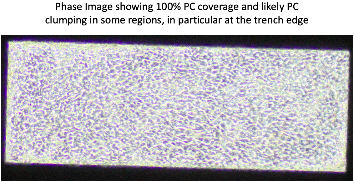
Please note that in this example experiment, BPLCs grew too 100% confluent quickly, and had regions with pericyte clumping. This is non-physiological, but was the best that I had to work with. Further, this data was acquired to compare basement membrane composition on cells exogenously-treated with ApoE3 or ApoE4. There was no clear difference between treatments, and this post is focusing on methodology, rather than a biological question.
Results

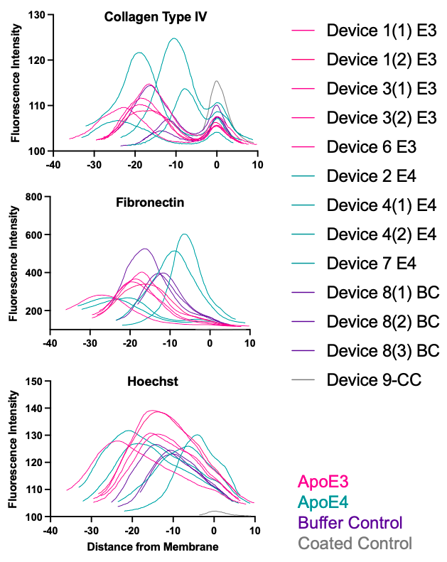
By extracting fluorescence across the z-stack for each component and normalizing the z location to the membrane, we can obtain plots of each BM component and where they localize in the µSiM coculture model. I believe we can use this data to differentiate EC- and PC-produced BM. We could potentially use it to evaluate relative thickness and variability of PC-produced BM. However, this depends on quality of pericyte layer and may be challenging. I am hesitant to use the data to quantify amount of BM production due to the many challenges of quantifying fluorescence intensity data.
Method for Extracting, Normalizing, and Plotting Fluorescence Data
Step 1: Extract z-axis profile data for all channels
Using FIJI (ImageJ), plot the z-axis profile for each channel and save the data as a .csv file.

Step 2: Determine membrane location
While it is probably easiest to set the membrane location as zero during imaging using the piezo stage, I did not plan for these analyses during image acquisition. Instead, the membrane location is different for all images. My work around has been to use the Col IV peak under the EC layer. I find the micron location associated with the second peak for each image. On the z-axis profile, select “List” (green boxes) and scroll down near the bottom. Find the [micron] value associated with the maximum mean on that second peak (black highlighted line).
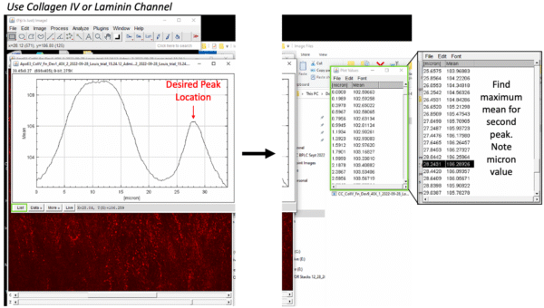
However, this peak is actually slightly above the membrane location. Further, it is possible different treatments will degrade this layer. An alternative would be to locate the region where the pericyte nuclei begin to fade out and endothelial nuclei begin to fade in. This is more subjective, but may be more reliable in future studies. Below are images showing the z plane in the pericyte layer (left), on the endothelial layer (middle), and at the transition between the two layers, i.e. at the membrane (right). The micron value or slice number can found at the top of the image.

So far, both methods determine very similar membrane locations.
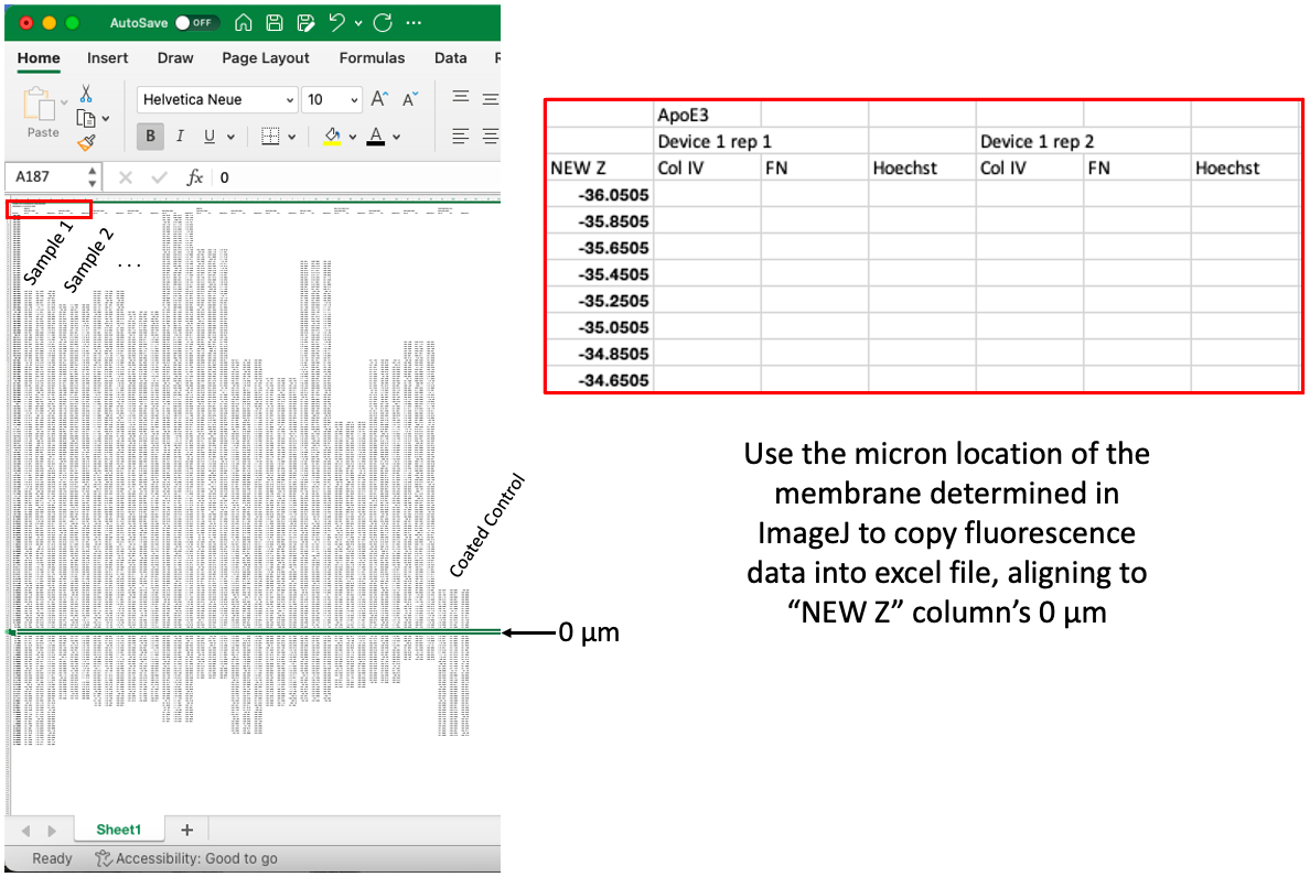
Step 3: Compile all data on excel, aligning each image’s 0 µm
There is likely an easier way to do this, but so far I have been copying the fluorescence data into excel from the .csv files. I drag the data from each image (all channels), down to a “New Z” column, where the I match the micron location of the membrane to “0 µm” in the New Z column, which is a new column of locations set 0.2 µm apart. You will notice that each sample has a different start and stop, but this makes it easier to copy into GraphPad Prism.
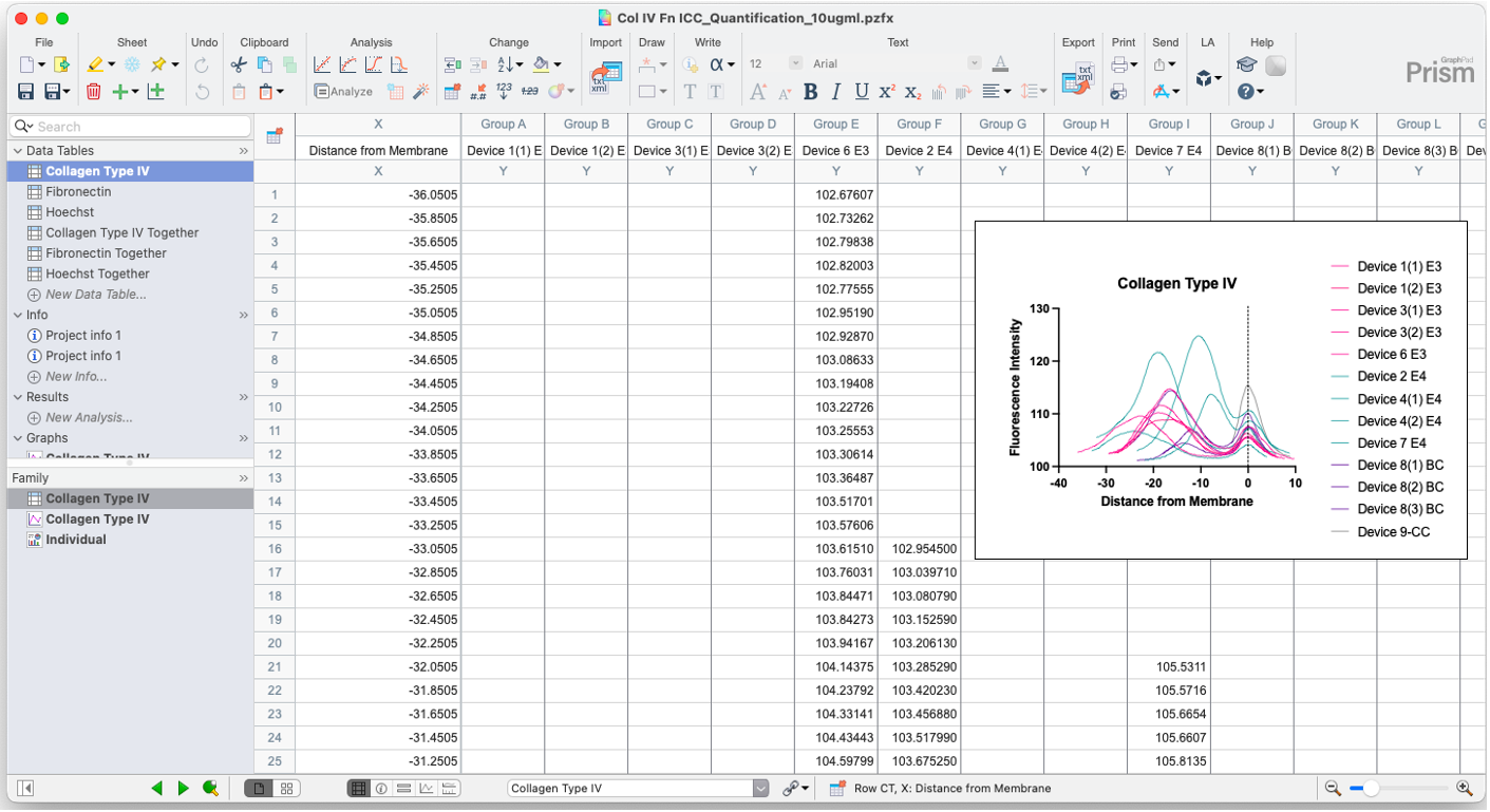
Step 4: Plot data on GraphPad Prism
Copy data into GraphPad Prism, making a new XY data table for each marker (You can ignore the “Together” Tables in the image below). Plot the data with separate lines for each group. I color coded treatment groups to match each other (exogenous ApoE3 in pink, exogenous ApoE4 in teal, buffer control in purple, coated control in gray). I do not run any statistics on the data, but use this as a visualization tool.
Conclusions
For now, I think we can use the plots to differentiate EC- and PC-produced basement membrane. It is clear that Col IV has two peaks, whereas FN generally only has one large peak. I have only tested laminin on EC monoculture controls, but there was clear deposition of a laminin layer (I used a polyclonal antibody). We will need to test this in coculture still, and could distinguish between types of laminin for a better understanding of the BM produced in our model.