WEKA-Based Pore Counting Analysis of TEM Images
Summary
There’s a lot to be desired in counting pores in grayscale images, especially when the contrast differences are low. A human eye is usually much better at picking out slight differences in contrast, and this can mean the difference between an open and closed pore. Differences of 5 nm can be significant in certain applications; 5 nm of material that fails to be removed may cause a wafer to have 0% porosity. However, the techniques (machine learning WEKA pixel classification and segmentation) that I’ve used to try and automatically count microplastics can be similarly used to establish what is an open pore and what is not. These results are promising for replacing the TCgui pore processing software.
**Update 3/21/2020** The software files are now obsolete, find the current processing software on the resources page.
Software Files
Obsolete:
Version 1 WEKA Pore Processor and Classifiers
This includes my imageJ macroscript to process images, as well as examples of classifiers I’ve trained.
Version 4 WEKA Pore Processor and Classifiers
This version will create an organized output based on the input TEM directory. Right now, only classifiers for 8900x, 13500x, and 17500x have been trained.
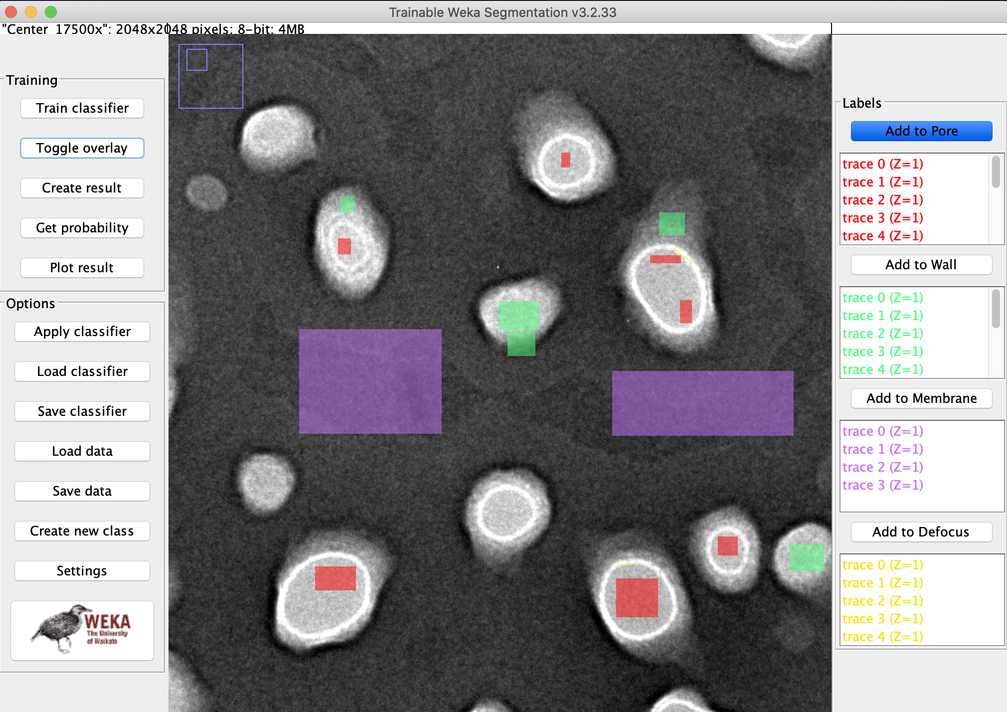
Classifier Training
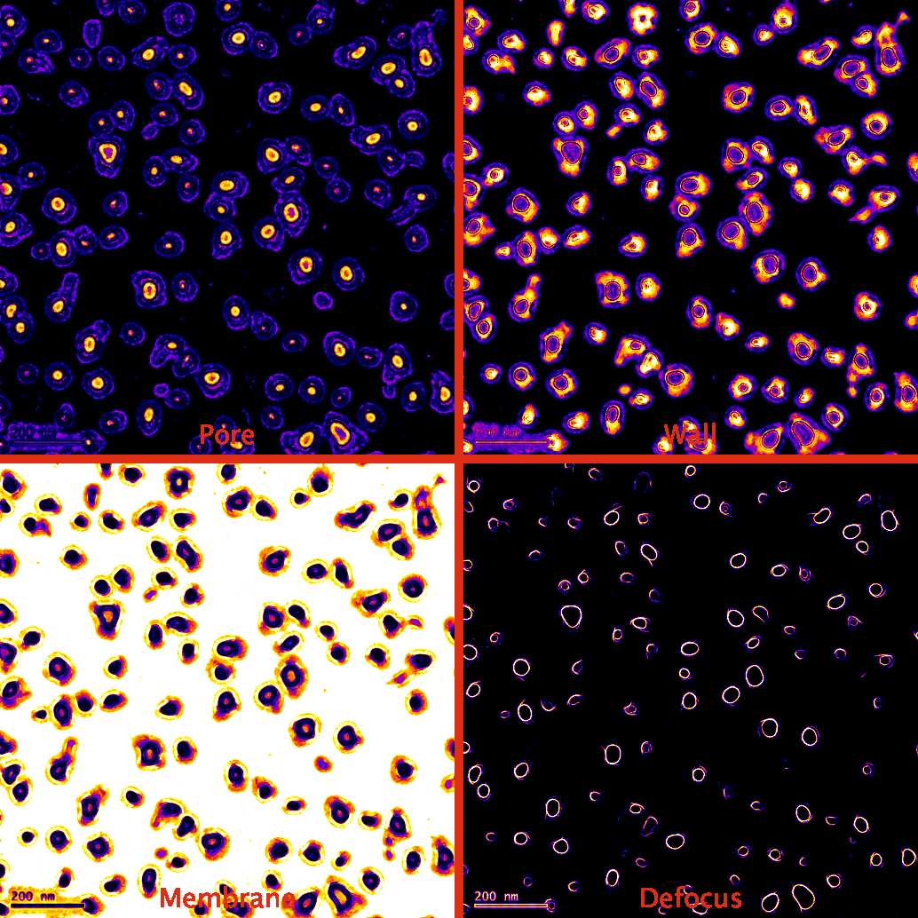
I chose 4 classes of object to recognize: The membrane area, the void space of the pore, the sidewalls of the pore (or divoted regions), and the defocus ring around the sharp edges of the pore.
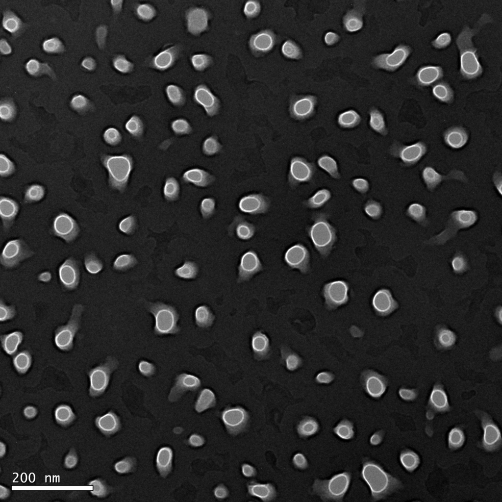
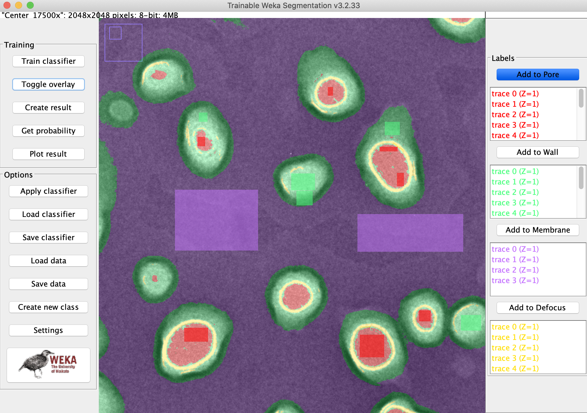
Example Results
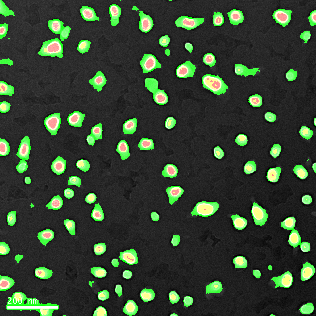
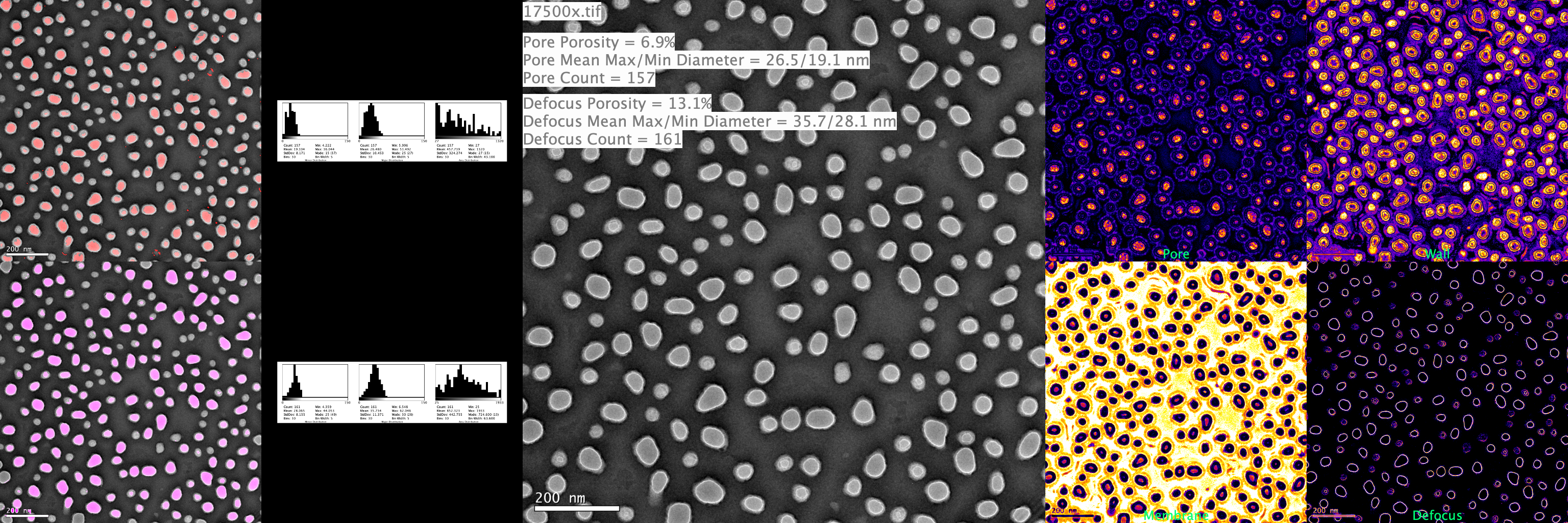
The macro takes the raw probability distribution and attempts to analyze the image with two different strategies.
- Use the void space of the pore to count pores.
- The image is denoised, then filled to provide contiguous surfaces for pore counting, porosity estimation.
- This method works better when there are fewer pores in the image (more void space is represented relative to the defocus ring)
- Works better on edges
- Use contiguous defocus rings to count pores
- The image is denoised, then the ring structures are filled to create a contiguous structure for pore counting, porosity estimation
- This method works better when there are clear defocus ring edges; incomplete rings will be thrown out and not counted.
- Works better on unevenly etched membranes as the rings provide a pore/non-pore classification.
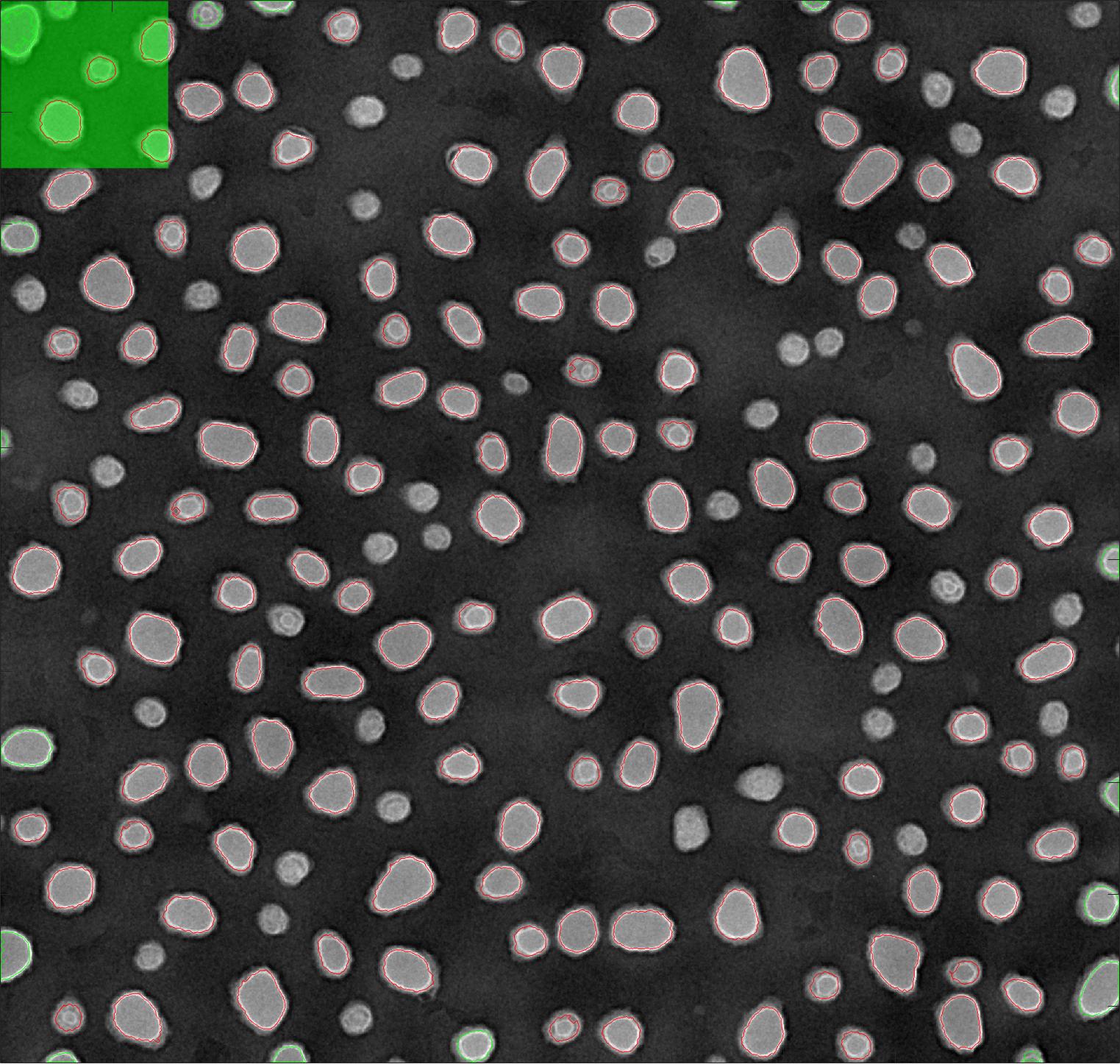
From here on out, it is trivial to count pores using ImageJ’s analyze particles function. If we can create more precise classes and segment what is an open pore, our results will improve.
***The macro only counts pores with circularity = 0.6-1.0 and has area greater than 25 pixels^2*** If you want to change this parameter, adjust lines in the code that say
run(“Analyze Particles…”, “size=25-Infinity circularity=0.60-1.00 show=Masks display summarize”);
Specifically, the void region of the pore at higher magnifications is very sensitive to the circularity parameter, which can lead to lower counting stats than the coloring would indicate.*****
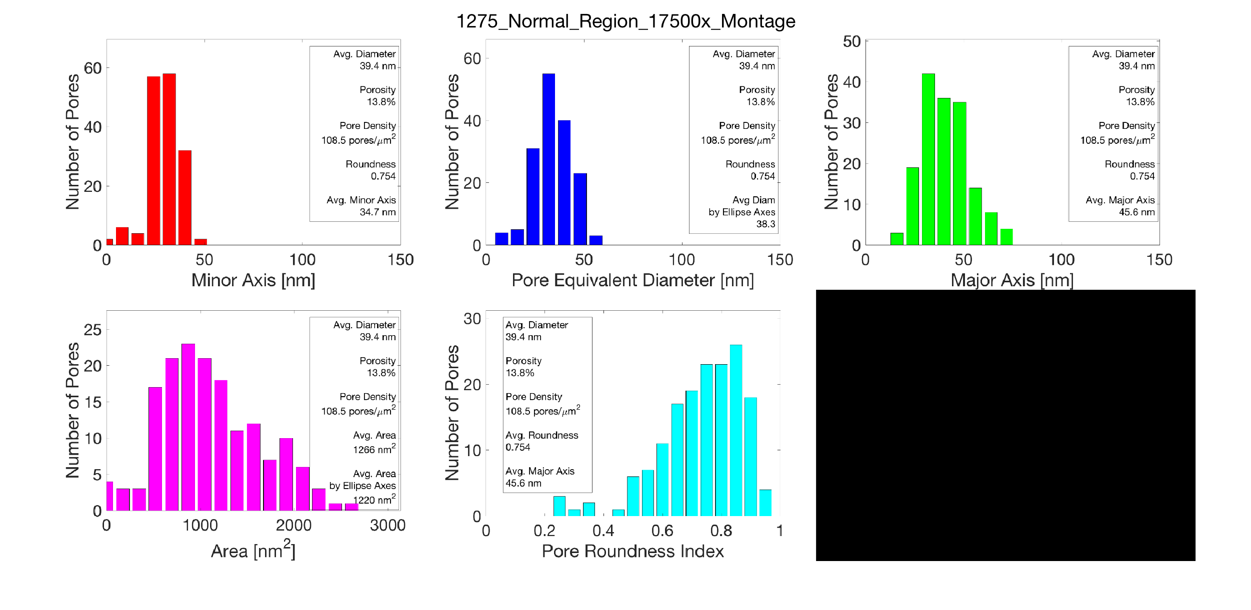
Comparison with Old Manual Stats
Here’s an example from 1275 NPN.
Example Output Folder
