Experimental Validation of the ECMO Model
Two of my recent posts have dealt with my efforts to model ECMO and to experimentally validate this model. This post will describe the key change I made to my experimental system since my last post and describe my efforts to recreate the experimental results with my model — successfully!
In an turn of extraordinary providence, we recently learned that the hemodialysis device Fresenius provided for the senior design program comes equipped with a spectrometer designed to measure hematocrit and oxygen saturation in blood as it flows through the dialyzer in real time. The ability to measure oxygen saturation during an experiment, rather than by sampling afterwards, solves every problem I was having with my ECMO experiments. Not collecting samples of the hemoglobin solution removes just about every opportunity for error to be introduced into the system, and having a robust and well-calibrated oxygen saturation reader eliminates the possibility of incorrect interpretations of the absorbance spectrum data. It’s perfect.
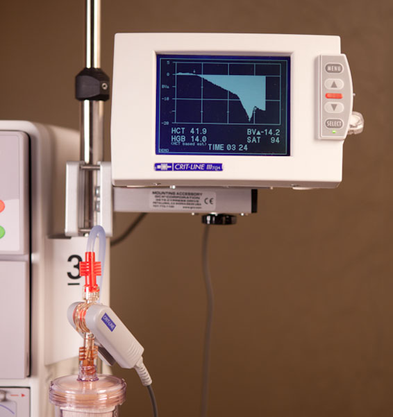

The Crit-Line III sensor functions by making readings of the absorbance of blood flowing through a special cuvette tube, shown on the right. The adapter on the bottom left of this image is of appropriate size for a luer connection, and the other adapter is a proprietary format that screws into Fresenius fiber bundle dialyzers, but I connected it to a standard blunt needle using a plastic tube adapter. The system has a couple small quirks; it can only make measurements on blood (if it doesn’t recognize the liquid in the cuvette as blood it returns an error rather than a measurement) and even hemoglobin solution won’t work (presumably it would work, if you could make a hemoglobin solution as concentrated as blood without it precipitating out…). Furthermore, the cuvette must be oriented upright as shown in the photo on the left, or it won’t fill properly.
So with the help of resident phlebotomist Margaret Youngman and a few vials of her kindly-provided blood, I performed an ECMO experiment with the Crit-Line. The experiment was set up very much like it was described in my previous post, but no pre- or post-ECMO collection chambers were included and a Crit-Line cuvette was inserted into the line both before and after the membrane. The outlet of the line was left open and submerged in water, and the following experimental parameters were used:
- Blood flow rate 0.36 mL/min
- 1 mm gasket height for blood channel
- 100 mmHg gage pressure of pure O2 on the other side of the membrane
I deoxygenated the blood for one hour before beginning the experiment. Because blood is so rich with hemoglobin, it takes much longer to deoxygenate than a relatively dilute hemoglobin solution, but bubbles could be seen evolving out of the blood for quite some time. I then began the flow and made recordings of the O2 saturation reported by the Crit-Line at both cuvettes at regular intervals until a clear steady-state had been reached. The recordings were as follows:
| Time (min:sec) | 2:20 | 5:30 | 6:50 | 8:30 | 9:50 | 11:20 | 13:30 | 16:00 | 18:00 |
| Pre-ECMO | 65 | 65 | 64 | 65 | 65 | ||||
| Post-ECMO | 74 | 74 | 72 | 72 |
While the Pre-ECMO saturation is quite stable, there’s some decline in the Post-ECMO saturation after a while. I attribute this to the effect of atmosphere in the line being displaced by the blood — though the outlet was submerged in water, the tubes and cuvettes were initially filled with a small volume of atmosphere that would’ve had some effect on the oxygenation of the early blood that eventually pushed it out of the system. Therefore, I trust the later value of 72% saturation to be the “true” value.
So, what does the model predict? First, allow me to describe the model a bit more and discuss some subtleties.

This model has been broken up into five domains, which I’ve labeled (a) through (e): four for the blood channel and one for the other side of the membrane. Domain (a) is the gas side of the membrane, and is described by a simple diffusive space (no convection) filled with oxygen at the appropriate concentration for 860 mmHg of pure oxygen gas at 20 C (that’s 100 mmHg gage pressure of oxygen — 100 mmHg plus 760 mmHg (= 1 atm), so 47 mM). This region is very coarsely meshed because nothing interesting happens here. (b) is where the blood inlet is, on the right side, but because there’s no oxygen in this region and thus no reaction, it is also meshed coarsely. Domains (c) through (e) are meshed very finely because the reaction occurs here, after the membrane, and in particular the upper boundary is given a very fine boundary-layer mesh to accommodate the particularly high concentration gradients at that edge. These domains are really all the same, but are divided for analysis reasons: the output I’ll be measuring is the area-average oxygenation of the blood within domain (d). I choose this rather than the line-average oxygenation at the outlet because there’s some significant error associated with the edge of a mesh (i.e., at the edge of a domain) as can be noticed with a keen eye on the snapshot.
While I initially took the model provided by Prof. Clark at face value, some investigation into the parameter values we employ is due. There are four parameters that govern this model: total heme concentration (NT), partial O2 pressure at 50% saturation (P50), the Hill Equation constant (n), and the Bunson solubility of oxygen in water (Buw). Prof. Clark’s ‘Oxygen Delivery from Red Cells’ provides values for these parameters as they apply to the space within a red blood cell at 37 C, but my application is to whole blood at 20 C. Therefore, I used some different parameters:
- NT: Clark was investigating the space inside a red blood cell, which is extremely dense with hemoglobin. Whole blood also includes acellular plasma volume, so we need a different value. Fortunately, the Crit-Line measures hemoglobin in real time as well, and in my experiment Margaret’s blood was measured to have 15 g/dL of hemoglobin — or 60 g/dL of heme subunits.
- P50: This value depends heavily on temperature — otherwise identical samples of blood at 37 C and 20 C have extremely different oxygen dissociation curves. A rather ancient paper [1] provides the basis for my estimation of 6 mmHg at 20 C (down from Clark’s 26.4 mmHg).
- n: The hill equation provides the basis of Clark’s model of hemoglobin reaction, and indeed most models of this process. The parameter n describes the cooperativity of binding as we’ll discuss more shortly, but its exact value is subject to empiricism — Wikipedia describes the appropriate value as being between 2.3 and 3.0 (without citation, so who knows where this came from). Clark uses 2.65. To cover all bases, I ran simulations at 2.3 and 3.0 and observed a change of less than 0.1% saturation between the two.
- Buw: This parameter describes the solubility of oxygen gas in water (and, by way of a simple linear relationship, in blood) and depends on temperature. Clark uses 1.186E-3 mol/(L*atm) whereas I found a source reporting 1.3 E-3 mol/(L*atm) at 20 C [2], so not much difference there.
This model must be solved in a transient (time-dependent) manner because the extremely high gradients caused by the rapid reaction term make steady-state solutions impractically difficult. Thus, the output of this model is a measurement over time:
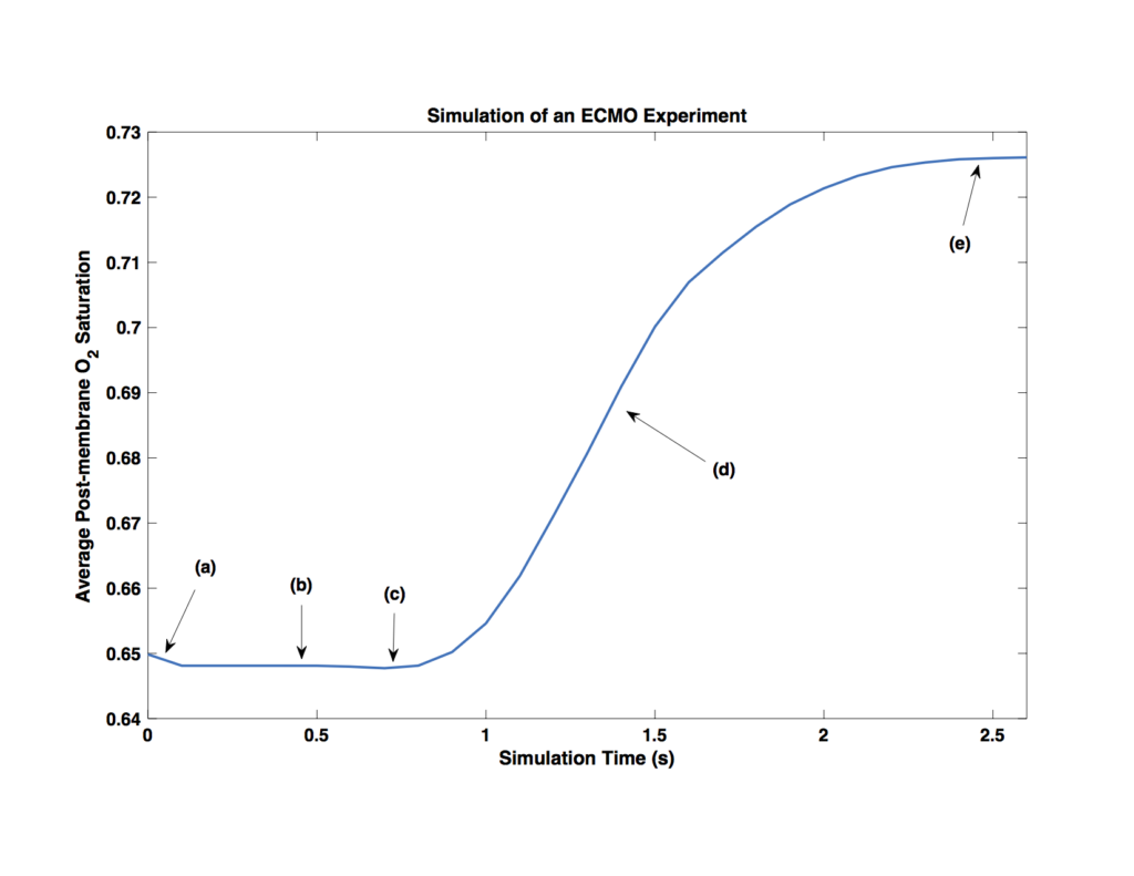
Once more, this is the area-average oxygenation within domain (d) over time. I’ve indicated five elements in this plot that I want to explain, because I think it’s quite interesting!
(a) The initial saturation of the blood was set to 65%, with no oxygen in the solution. Of course, this means that the first thing the model will do is go to equilibrium between oxygen bound to the hemoglobin and oxygen dissolved in the blood. This appears as a small dip in the initial saturation and in effect means the initial saturation was set to something like 64.8%.
(b) This region is simply waiting for the more oxygenated blood being produced near the membrane to flow to the measurement region.
(c) A careful eye will notice a slight dip in saturation here, just before the rising saturation. I believe this harkens back to the cooperativity of binding modeled by the Hill Equation. What this means is that hemoglobin that is bound to some oxygen has an increased affinity for more oxygen. Though we’re not modeling individual hemoglobin molecules here, the effect is still captured in ensemble by increasing the rate of reaction slightly in regions of higher saturation. This little dip is what happens when you measure the saturation in a region adjacent to a region of relatively high oxygenation. The increased affinity in the high-oxygen region depletes nearby regions by stealing their oxygen! This effect has no bearing on the macro-scale behavior of the system, but it’s pretty neat all the same.
(d) This region is where the oxygenated blood is convecting into the measurement area, before steady state has been reached.
(e) Finally, we have steady-state oxygenation! The final value is about 72.5%, which is very much in line with the experimental value. In fact, I would expect this prediction to be slightly larger than the experimental value because this two-dimensional model doesn’t account for the fact that in the experimental system not quite 100% of the channel width is exposed to the membrane. This may account for the extra 0.7% saturation (0.5% at the top end, plus the initial saturation was 0.2% lower than intended).
Update 5/25/16: A keen observer might notice that while my experimental system has a 2-mm-long membrane, it’s 3 mm in my simulation. An embarrassing oversight. Fortunately, rerunning the simulation with the proper membrane dimension only reduced the final saturation to about 71.9% — even closer to the experimental result. The smallness of this change in saturation relative to the change in membrane area makes some sense given that by the time the blood reaches the last millimeter of membrane, its local saturation next to the membrane is already 100% and therefore much less oxygen is demanded than was the case upstream.
So that’s a wrap! While this experiment was only (successfully) performed once I believe the evidence is very convincing that the model is accurately describing ECMO and has therefore been experimentally validated. I’ll be writing this up as a chapter in my thesis, and perhaps we’ll publish it.
[1]: Barcroft, J. and King, W. O. R. “The effect of temperature on the dissociation curve of blood.” 1909. J Physiol. 39(5): 374–84.
[2]: Sander, R. “Compilation of Henry’s law constants (version 4.0) for water as solvent”. 2015. Atmos. Chem. Phys. 15: 4399–981.