Particle Tracking in Tangential Flow Analysis
When we are trying to optimize the capture of exosomes in the tangential flow system, it is important to understand how particles are behaving in the flow. Initially, we tried to do this last summer by looking into the particle tracing package for COMSOL, but that required a complete overhaul of the software (a new purchase and everything) so we decided to wait on that module. Since then, Tejas and I have worked on a model for retaining a particle on a pore based on the forces acting upon that particle. Additionally, I have thought about developing an analytical model for our system and then applying this to the particle using the Maxey-Riley equation for particle tracking. However, this method involved a highly complex partial differential equation that took into account the history of the particle’s position, making it almost impossible to solve without some serious computational power.
In order to try to still model the position of the particle as it experiences flow, there was one way that we could potentially do this very simply (relatively). By making the assumption that the particles are sufficiently small that they will behave according to their immediate environment (meaning the flow conditions do not vary significantly (I know that term carries statistical connotation, but please pardon my usage in this case (also pardon the parenthe-ception)) around the particles) and will follow the local streamline at their immediate position. In addition to this, we would be able to observe diffusion effects on the particles, which would allow them to traverse streamlines, potentially allowing them to be transferred to streamlines that go towards the membrane when they would have otherwise flowed out of the system. The only question then was: where does the streamline data come from?
Conveniently, our friend COMSOL can help us out in this matter. After we run a simulation in COMSOL, it is possible to export velocity field results into a text file and then import these into an Excel spreadsheet. The data corresponds to the velocity components of each and every node in the meshed geometry and one can therefore imagine that there is a rough solution or a more refined solution to be had for these analyses. The solution that we arrive at would therefore be highly dependent on the mesh size: a more refined mesh would give us a more accurate representation of the particle behavior. The velocity field data can then be used to find the localized displacement of a particle at a node, using the local velocity. The displacement can then be applied to the original position and based on the new location, new velocities can be found and a new displacement can be calculated and so on.
Using a model I had developed last summer for our membrane with actual geometry pores (I modeled hundreds of discrete nanopores in a 100 μm long x 20 μm tall channel.), I extracted the velocity field data and imported it into an Excel spreadsheet. I then, with the help of Jim, wrote a code to find the nearest node to a desired input node. From there, I went and asked for Henry’s assistance (because my Matlab is quite messy, so helped me refine it and make it elegant) and we were able to generate a script that tracked the position of any number of particles positioned at random initial positions by this method. This resulted in a plot that basically represented the streamlines with the system, as shown in Figure 1.
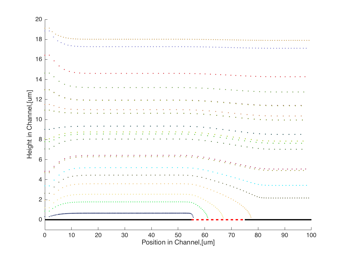
Figure 1: Particle position in the geometry without active diffusion. The particles follow the streamlines in this system. The representation of the membrane and inactive areas may be slightly off.
The next most important thing was to then add in diffusion. Since we have laminar flow, diffusion is an important part of our system and therefore, must be accounted for. This was done with the Stokes-Einstein equation for calculating the diffusivity of our particles (we can vary the radius of the particle) and then determining the mean squared displacement for each particle. The particles will also experience a random, normally distributed step length which was confirmed as shown by the histogram in Figure 2.
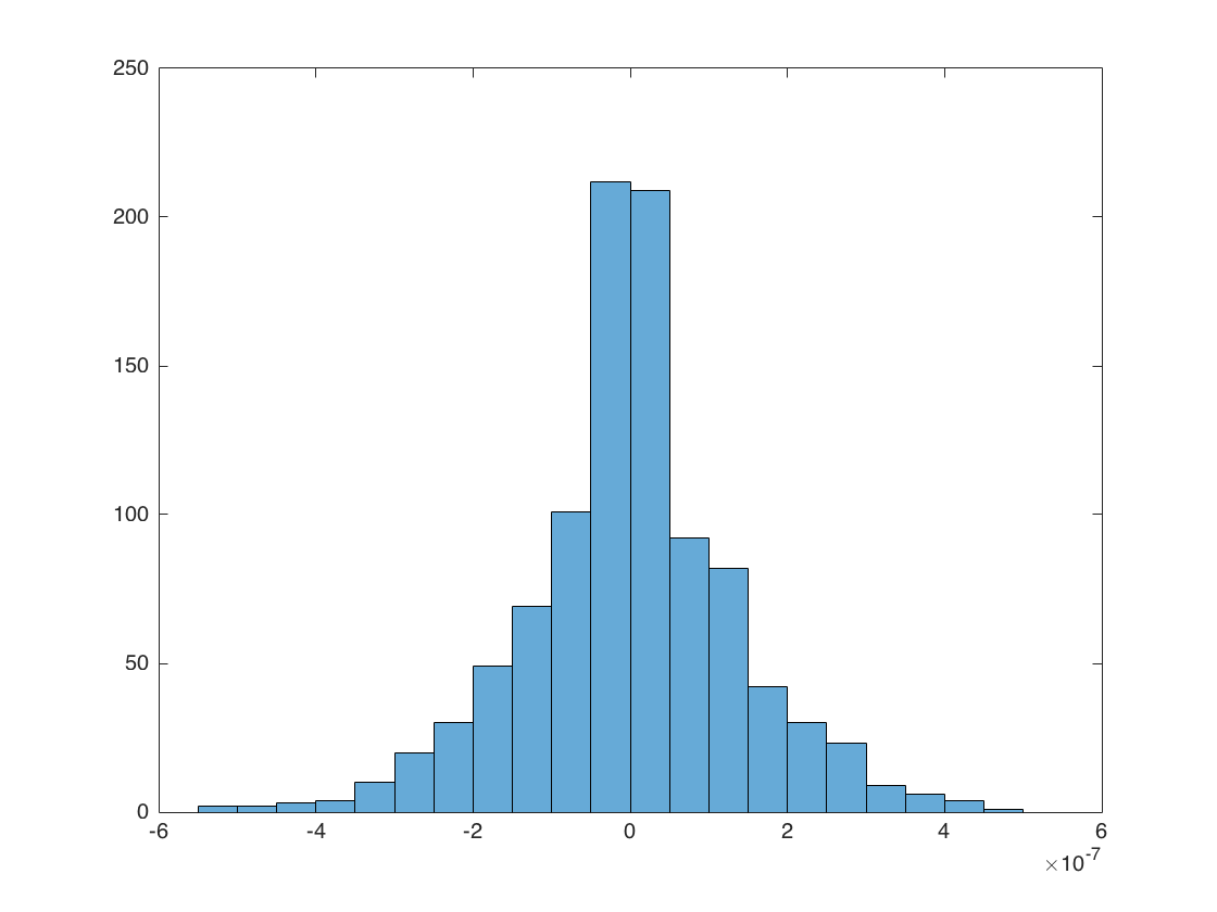
Figure 2: Normally distributed random step length for the diffusion of our particles (units are m).
Adding this in to the model, we then get the result shown in Figure 3.
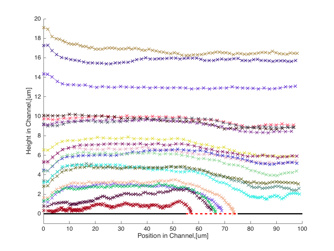
Figure 3: Particle position with diffusion in the model geometry.
This was a very nice simulation, but it might not represent our actual geometry. In that case, I developed a model with the exact dimensions of our chips and made the membrane a porous substance with a permeability matching our membranes. As we can see in Figure 4 and Figure 5, with this geometry the effects of diffusion were very, very small and particles pretty much followed the streamlines.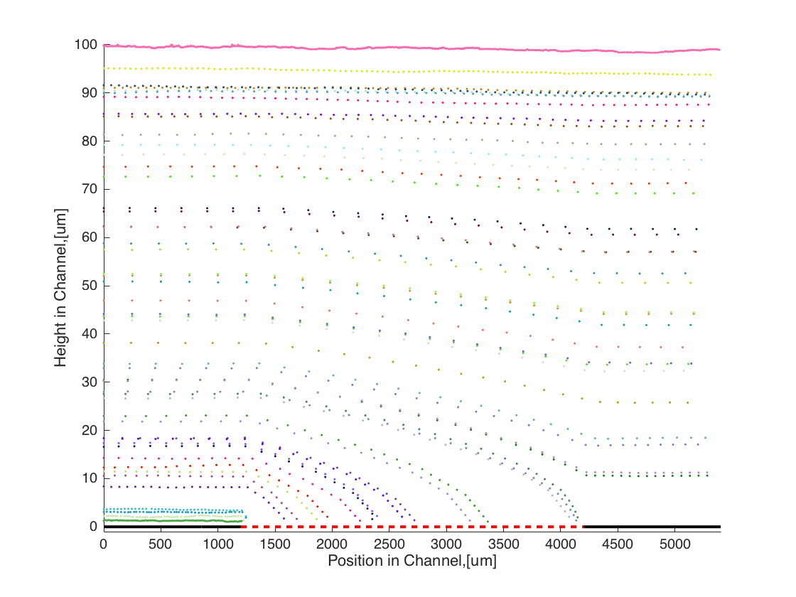
Figure 4: Actual geometry particle tracking. The capture layer for a 10/2 flow configuration with a 100 μm tall top channel is approximately 30 μm.
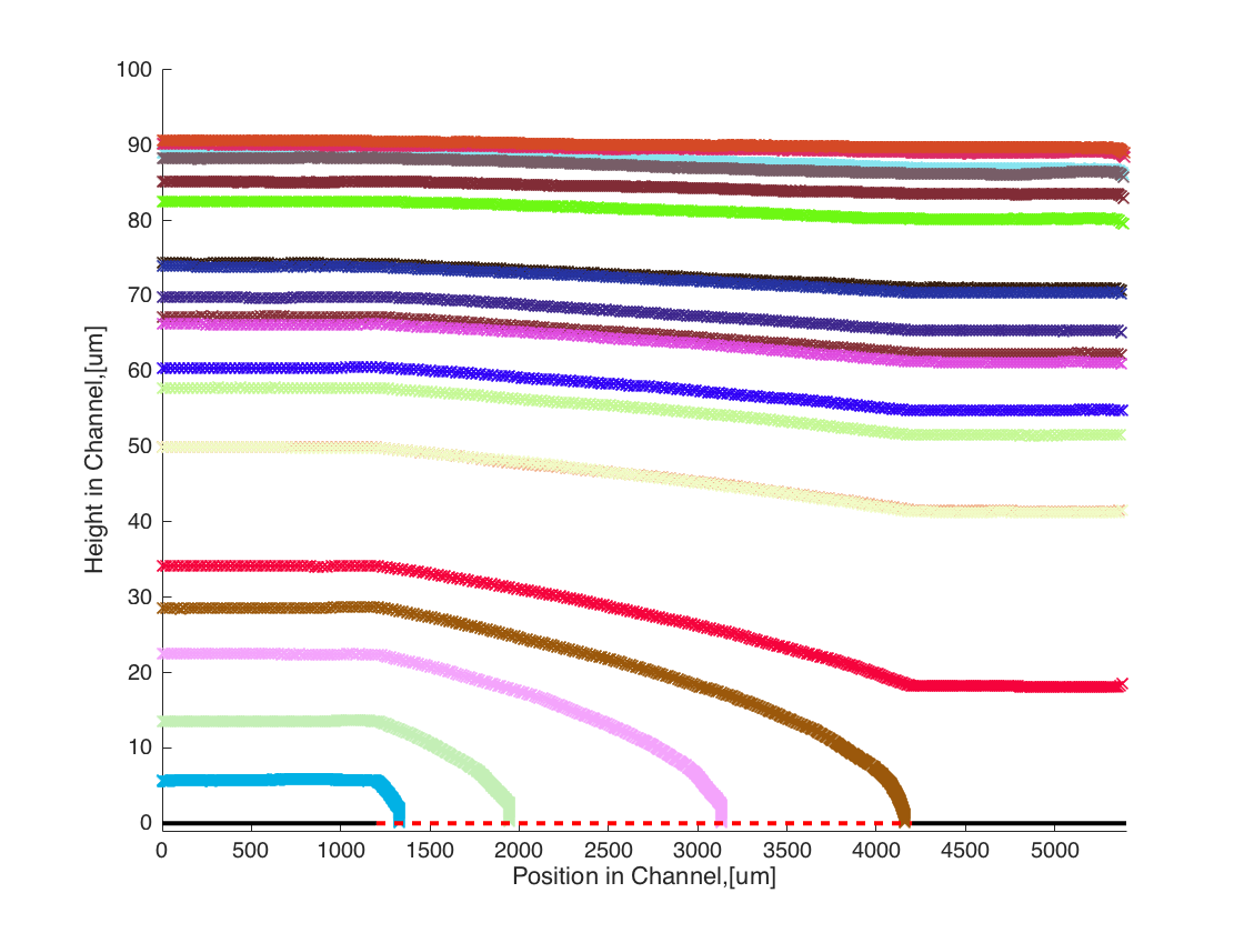
Figure 5: This is the same thing as Figure 4, with different particle starting positions and a different data marker for easier visualization.
This model and analysis are very convenient for determining the appropriate conditions for capturing exosomes, namely in helping to understand that height at which particles will be likely to interact with the membrane if they are positioned at or below it. It also helps us to see that for the lifetime of these particles in this system, diffusion does not really play any affect in helping to capture the particles. In fact, a quick Peclet number analysis showed that our Peclet number was on the order of 7,000, so this conclusion makes sense. I am currently running a COMSOL parametric sweep simulation where I am varying the flow rate in each channel from 1-20 μL/min in 1 μL/min intervals and this process will take several days (as I also have a very fine adapted mesh for more accurate results). Once this is complete, I will have a database flow rates that we can then plug into the model and gather statistics on. I will also be adding another parameter, which is the height of the channel, so that we can have the most robust analysis possible.