Electrostatic Effects on Convective Flux of Nanoparticles: A Mathematica/Matlab Implementation of W.M. Deen’s Model
UPDATE: I have since ported the program into Matlab. If you open the following zip document(Archive) you can run Find_Sieving_Coefficient. You can select a results file and after ~5 minutes the expected sieving coefficient for the pore distribution is spat out.
Using Wolfram Alpha’s Mathematica programming language, I’ve implemented an amalgamation of different mathematical models to model the transport of charged gold nanoparticles moving through a charged pore. Infuriatingly, WordPress doesn’t allow Mathematica notebooks to be uploaded, so here’s a link to it hosted on my google drive (also a text file uploaded to the blog: Sieving model dynamic 3.14.14) EDIT: code is now uploaded to the cloud @ http://drive.bbe.23a.myftpupload.com/index.php/apps/files?dir=/Shared/NRG/Code/Sieving%20Models . If you’re trying to understand the theory behind the separation, I produced a cleaner copy that sacrifices the dynamic updating and the ability to plot for ease of understanding (text file: Sieving Model static). If you do not have a copy of Wolfram, it’s available for free for everyone affiliated with HSEAS (and apparently @urmc.rochester.edu email addresses work too for the verification). They’ll make you jump through a few hoops, but it took me no more than twenty minutes to get it running on my computer. Wolfram allows for dynamic modulation of output, so I’ve crafted the following user interface:
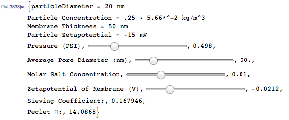
The sliders are useful for getting an intuition about what’s happening as various parameters are tweaked.
I chose mathematica because of a promotional video that told me that it was possible to upload mathematica code to the cloud, and anyone with the link (regardless if they had mathematica) could interact with a user interface similar to the one I put together. Unfortunately that functionality hasn’t been rolled out yet. So since not everyone will have access to the dynamic program, I’ve put together a few representative charts.
For the following, we assume a ‘standard separation’ with the following inputs:
particle diameter: 20 nm
particle concentration: .25 * 5.66E-2 (4 to 1 dilution of BBI values from their website)
average pore diameter: 50 nm
membrane thickness: 50 nm
transmembrane pressure: 1 psi
molar salt concentration: 10 mM
particle zetapotential: -0.015 V
membrane zetapotential: -0.020 V
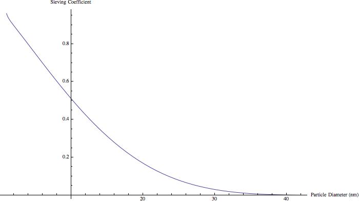
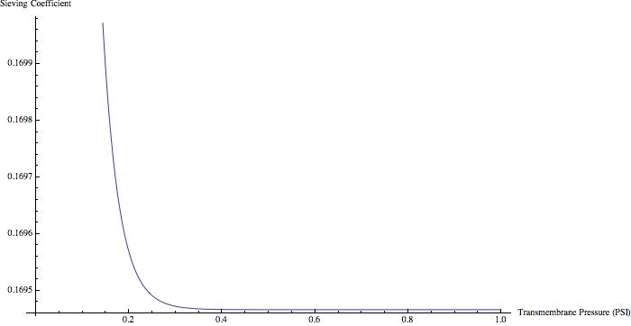
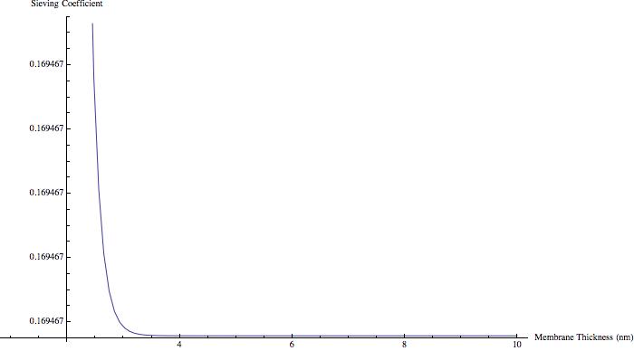
Each parameter is then tweaked and plotted against the resultant sieving coefficient.
Average pore diameter v. sieving coefficient:
Transmembrane pressure v. sieving coefficient:
Membrane thickness v. sieving coefficient
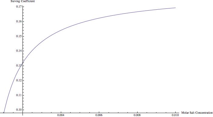
Molar salt concentration v. sieving coefficient:
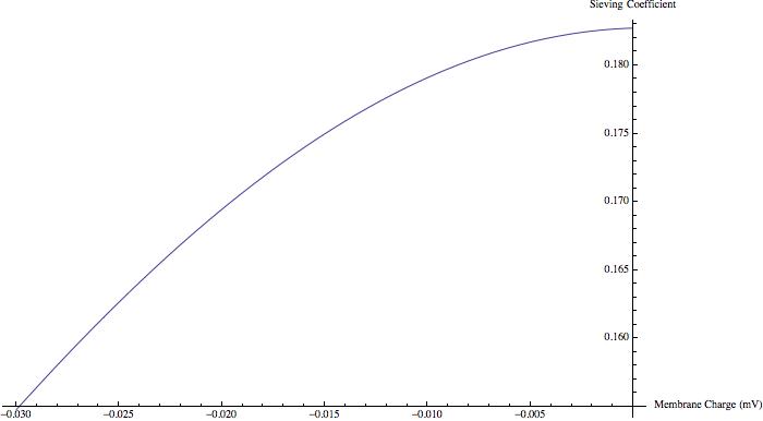
Membrane surface charge v. sieving coefficient:
The following comes (with some edits) from my qualifying exam proposal:
Filtrate concentration of gold can be understood as the ratio of solvent (water) flux to solute (gold) flux through the membrane. Solvent flux can be found from the applied pressure using the Dagan Equation:
![Latex Q = \frac{\Delta P r^3}{\mu\left[ 3 + \frac{8}{\pi}\left(\frac{l}{r}\right)\right]}](https://staging.nanomembranes.org/wp-content/ql-cache/quicklatex.com-484fe23b213a12f35e64ec9f1c86aa24_l3.png "Rendered by QuickLaTeX.com")
(where  ,
,  ,
,  , and
, and  are the solvent flux, solvent viscosity, pore radius, and pore length, respectively) which is an extension of the Hagen-poiseille equation to pores that cannot be approximated as infinitely long. Solutes at least a few times bigger than the solvent molecules (gold can be as small as 5 nm diameter; a water molecule is
  0.25 nm long) can be treated as Brownian particles subject to hydrodynamic resistance. For simple diffusion (i.e. spherical particles in an unbounded fluid) the solute flux is given by Fick’s Law of Diffusion as
  , where
  is the diffusivity of a solute molecule as given by the Stokes-Einstein equation,
  is concentration, and
  is distance from the pore. Because of steric and electrostatic interactions, the free diffusion of particles is `hindered’ within the narrow confines of the pore, so that the diffusive term is actually
  , with a diffusive hindrance factor (also called the enhanced drag)
  . Similarly, purely convective transport can characterized by
  , with
  representing the bulk flow and
  the convective hindrance factor (also called the lag coefficient). Solute flux is a sum of the diffusive and convective components of flux through the membrane:

Deen (Hindered transport of large molecules in liquid-filled pores – pdf hosted by blog) derived the following system of equations to describe solute flux  :
:



![Latex \langle N \rangle = W\langle V \rangle C_{\text{feed}} \frac{[1-(C_{\text{filtrate}}/C_{\text{feed}})e^{-Pe}]}{1-e^{-Pe}}](https://staging.nanomembranes.org/wp-content/ql-cache/quicklatex.com-68d08da028327cf7b77bc08ef6220ac9_l3.png "Rendered by QuickLaTeX.com")
where  is the dimensionless radial position,
  is the Peclet number (the ratio of convective to diffusive transport in the system),
  , and
, and  is the boltzman energy.
  and
and  are two hydrodynamic functions that modify the diffusive and convective flux (respectively) due to steric and electrostatic interactions. Note that the limiting cases for the last equation are
  for
for  and
and  for
for  .
.
You’ll notice that the filtrate concentration  on the right hand side of the equation, which is where the model begins to make assumptions that are more difficult to justify. To calculate the filtrate concentration of gold (which we need to calculate the diffusive flux) , we assume that there is no concentration polarization (no ‘traffic jam’ behind the membrane due to gold moving slower than water) and that the system is in steady state. If our solution is dilute, this is a fairly reasonable assumption – even though some gold is ‘rejected’ by the pore, it diffuses rapidly back into bulk solution and the concentration at the entrance approaches the concentration in the bulk. This rejection of gold is defined by the rejection coefficient
  which represents the fraction of gold that does not pass through the membrane, and multiplying this by our feed, or bulk, concentration of gold gives us the expected concentration of gold in the filtrate due to convection. This is then used to calculate diffusive flux across the membrane in the above equation. This is why the sieving coefficient is so high in the limit of low transmembrane pressure – the model calculates the diffusive flux across the membrane assuming that the concentration of the feed is fixed, and that the concentration of the filtrate is also fixed at 0. But in the low-pressure limit, we should be using Jess’s model anyways.
Additionally, the model currently uses the average pore diameter for all calculations. As we’ve seen generally in Dagan flow, the larger pores are disproportionately responsible for transmembrane flux, due to the no-slip condition of flow and the r^4 dependence on flow rate. As a result, the average pore diameter will likely significantly underestimate the sieving behavior of the system. This is easily fixed by running the program for each pore in the pore histogram output, but it will necessitate re-writing the program in MATLAB so it can interface with the pore image processor.
In Electrostatic effects on the partitioning of spherical colloids between dilute bulk solution and cylindrical pores (pdf, hosted on blog), Smith et. al. find

where  are the Cylinder radius, the solvent dielectric permittivity, the gas constant, the faraday constant, and the Gibbs free energy, respectively.
  at constant surface charge represents the change in free energy between a charged particle in solution and the charged particle within a charged pore, and is given as the following equation:

where  is the ratio of pore radius to debye length,
  ,
,  is the modified bessel function of the first kind,
  and
and  are the surface charge of the sphere and the cylinder, respectively, and when the dielectric constant of the metal is much higher than that of the solvent,
  can be approximated:
![Latex \Lambda \approx \frac{\pi}{2} I_0(\tau\beta) \sum_{t=0}^{\infty}\frac{\beta^t(2t)!}{2^{3t}(t!)^2}I_t(\tau\beta)\times\left[ \tau K_{t+1}(2\tau) + \frac{3}{4}K_t(2\tau)\right]](https://staging.nanomembranes.org/wp-content/ql-cache/quicklatex.com-7950fd6c1e33f681e97cb8d594af4fac_l3.png "Rendered by QuickLaTeX.com")
where  is the modified bessel function of the second kind. Note that and are both exclusively in the numerator of equation, meaning as either surface’s charge increase the associated change in free energy likewise increases. These numbers are found from the experimentally derived zetapotentials via the following formulas:


which I found in Jess’s thesis, but I haven’t yet been able to figure out where she found it. Further note that because the surface charges are additive, even if one of the surfaces charges were zero there would still be an electrostatic component to the difference in free energy. Only if both of the particles had zero surface charge would this expression go to zero. This expression is derived by describing a charged sphere and a charged cylinder using the linearized Poisson-Boltzman equation in both spherical and cylindrical coordinates (respectively), identifying the boundary conditions of the two systems of equations, and then performing a coordinate transformation to apply one set of boundary conditions to the next.
and G are interpolated from Paine and Scherr’s (Drag coefficients for the movement of rigid spheres through liquid-filled cylindrical pores – pdf hosted on blog) numerical simulations using mathematica’s standard Interpolation function. It’s important to note that Paine and Scheer assume that there is no electrostatic repulsion ( ) within the pore for the calculation of these values. Dechadilok and Deen examine electrostatic effects on both and ; they found that accounting for electrostatics did marginally change both values, but the greater impact of charge-based repulsion came from whether or not the particles made it into the pore in the first place. Since we are accounting for electrostatics elsewhere, Paine and Sheer is a reasonable approximation. Note also that extensive experimental evidence indicates that the viscosity of water in pores down to a size of
  does not deviate significantly from its bulk value, and we can thus treat viscosity as uniform everywhere in our system.
Wow. This will take a while to digest, but I’m glad its here!
Can you host on owncloud instead of gdrive?
Also talk to david about the trouble uploading to WP.
Code has been uploaded to owncloud @ http://drive.bbe.23a.myftpupload.com/index.php/apps/files?dir=/Shared/NRG/Code/Sieving%20Models