The New Concentration Polarization Model Turns Out To Be Difficult To Implement In Matlab
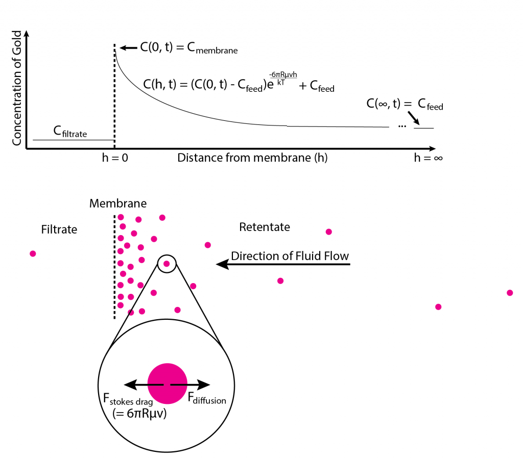
This is part three of a series of posts on constructing a mathematical model of the movement of gold through a porous membrane. In part one, I implemented William Deen’s mathematical model of the electrostatic and steric effects that contribute to whether a gold nanoparticle will translocate through a pore. The mathematica and matlab code I created made some beautiful graphs, but the theory did not match experiment, likely because concentration polarization was ignored. In part two, I expanded upon the naïve electrostatic model by including the localized concentration increase (which is a time-dependent Boltzmann distribution) called concentration polarization (illustrated concisely by the following image:)
In this post, I detail my first, failed attempt at trying to bypass the analytic issues that arose in part two (what I called the ‘recursive definitions’ of my key variables) by attacking the problem with brute force. The following is my matlab pseudo-code:
Time of separation = 200uL/(hydraulic permeability * active area * pressure)

CurrentTime = 0
%The first iteration needs to be a little different
gap =


![\langle N \rangle = W\langle V \rangle C_{0} \frac{[1-(C_{\text{filtrate}}/C_{0})e^{-Pe}]}{1-e^{-Pe}}](https://s0.wp.com/latex.php?latex=%5Clangle+N+%5Crangle+%3D+W%5Clangle+V+%5Crangle+C_%7B0%7D+%5Cfrac%7B%5B1-%28C_%7B%5Ctext%7Bfiltrate%7D%7D%2FC_%7B0%7D%29e%5E%7B-Pe%7D%5D%7D%7B1-e%5E%7B-Pe%7D%7D+&bg=ffffff&fg=000&s=0&c=20201002)


WHMIT = 0 + total gold in gap
CurrentTime = CurrentTime +

While CurrentTime < Time of separation
gap =
total gold in gap
WHMIT = 0 + total gold in gap
CurrentTime = CurrentTime +
Loop


![\star \langle N \rangle = W\langle V \rangle C_{\text{average}} \frac{[1-(C_{\text{filtrate}}/C_{\text{average}})e^{-Pe}]}{1-e^{-Pe}}](https://s0.wp.com/latex.php?latex=%5Cstar+%5Clangle+N+%5Crangle+%3D+W%5Clangle+V+%5Crangle+C_%7B%5Ctext%7Baverage%7D%7D+%5Cfrac%7B%5B1-%28C_%7B%5Ctext%7Bfiltrate%7D%7D%2FC_%7B%5Ctext%7Baverage%7D%7D%29e%5E%7B-Pe%7D%5D%7D%7B1-e%5E%7B-Pe%7D%7D+&bg=ffffff&fg=000&s=0&c=20201002)

Display “Sieving Coefficient = ”

The line with 


Because we’re using a finite number of intervals to evaluate the system, we can’t use the surface concentration to determine the flux through the membrane – if you used 

As the code currently stands, the previous 
Regrettable, this model does not predict sieving coefficients because of this ‘recursively defined variable’ problem.