Adding a Compressible Cake Layer to the Theoretical Model

In a previous post (linked here), I discussed a naïve way to incorporate concentration polarization into our theoretical model of the sieving of charged nanoparticles. Essentially, I considered the particles to be uncharged point particles that were subject to a force pushing them toward a surface (fluid velocity) and a force pushing them away from the wall (diffusion) that formed a perfect Boltzmann distribution. This is pictured below:

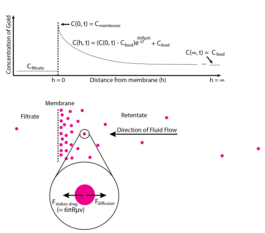
I implemented this in Matlab, along with a model of the charge-charge and hydrodynamic interactions between a pore and a particle, and got excellent agreement with experiment when I did so (post). But there serious issues with this approach that warrant taking a more mathematically rigorous approach to buildup behind the membrane. First, the fact that the model assumes the particles are points means that we get ludicrous values for concentrations at the membrane surface. In one simulation (link), I found that the gold concentration right at the membrane was roughly 10,000 M after a normal separation. We could account for this by figuring out the maximum density of particles before they aggregate and simply capping the concentration there (illustrated below)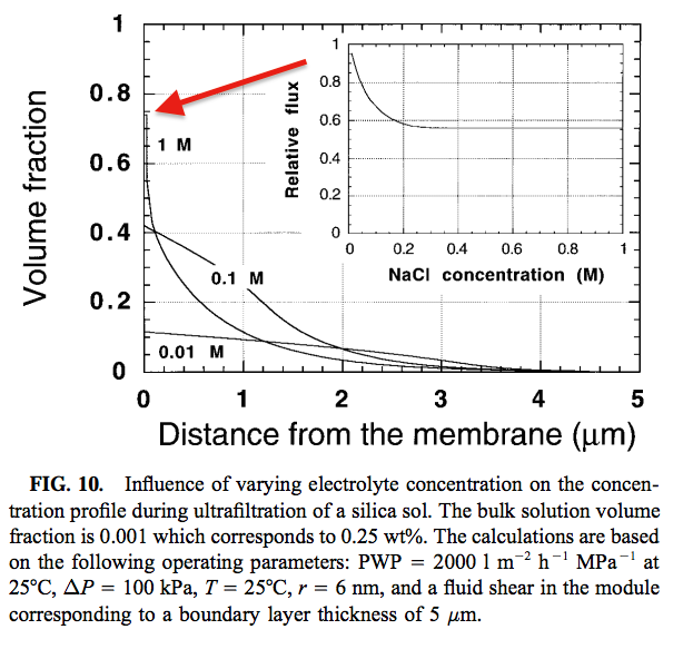

This ignores charge-charge interactions, which for gold nanoparticles are very important, especially because they are in very low-salt conditions. A more rigorous approach is detailed in Dynamic Ultrafiltration Model for Charged Colloidal Dispersions: A Wigner-Seitz Cell Approach (pdf). The authors use a hexagonal pack of spheres and a force balance that includes the electrostatic and van der Waals interaction of the spheres (while accounting for debye/counterion shielding), the compressive force of the driving pressure, and the diffusion of particles back into bulk solution. Using this description, the authors describe the concentration profile of particles at and above the membrane, which takes the form of the following three equations:

$\frac{dz}{dt} = -\frac{z^2}{V+A_mR_m\left(\frac{\rho_p}{c_b}-1 \right)(1-\varepsilon)\left(\frac{\mu}{\mu_a} \right) K_{\text{Happel}}}$

$\frac{dV}{dt} = z$

$p_2(t) = \frac{\mu R_m}{A_m}z+p_3(t)$

Where $V$ is the total volume filtered ( $m^3$ ), $A_m$ is the area of the membrane surface ( $m^2$ ), $R_m$ is the resistance of the membrane ( $m^{-1}$ ), $\rho_b$ is the particle density ( $\frac{\text{kg}}{m^3}$ ), $c_b$ is the particle bulk concentration ( $\frac{\text{kg}}{m^3}$ ), $\varepsilon$ is the fractional voidage of cake deposit (dimensionless), $\mu_a$ and $\mu$ are the apparent and actual (respectively) dynamic viscosity of the solvent ( $\frac{\text{kg}}{m *s}$ ) and $K_{\text{Happel}}$ is the permeability coefficient of a lattice of spheres as calculated in Happel’s 1958 paper ( $m^{-2}$ ). $p_2(t)$ and $p_3(t)$ represent the time-dependent pressure ( $N/m^2$ ) on the filtrate and retentate sides of the membrane, respectively.

Bowen et. Al solved this group of two first-order differential equations and one algebraic equation using a numerical predictor-corrector schema. As a matter of practical implementation, I’m having some difficulty in using the predictor-corrector methods, which work just fine for differential equations with only first derivatives, on this set of equations since there is pretty clearly a second derivative in the first equation. Because of that, I’ve begun to implement the simple high-salt approximation.

Darcy’s law gives us the hydraulic flux through a porous medium:

$Q = -\frac{\kappa A}{\mu}\frac{P_{\text{retentate}}-P_{\text{membrane}}}{L}$

where $Q$ is flux, $\kappa$ is the intrinsic permeability of the porous bed, $A$ is the area of the bed, $L$ is the length of the bed, and $P$ is the pressure.

Remember Dagan’s equation gives us the flux through a membrane:

$Q = \text{\# of pores}*\frac{(P_{\text{retentate}}-P_{\text{membrane}}) r^3}{\mu [ 3+\frac{8}{\pi}(\frac{l}{r})]}$

What’s tricky is that in both of these equations, we need to know $Latex P_{\text{membrane}}$ to find Q. The way that we solve this is to realize that the flux into the packed bed of gold and the flux out of the back of the membrane must be equal:

$-\frac{\kappa A}{\mu}\frac{P_{\text{retentate}}-P_{\text{membrane}}}{L} = \text{\# of pores}*\frac{(P_{\text{retentate}}-P_{\text{membrane}}) r^3}{\mu [ 3+\frac{8}{\pi}(\frac{l}{r})]}$

Or,

$P_{\text{membrane}} = \frac{-\frac{\kappa A}{L}P_{\text{retentate}} -\frac{\text{\# of pores}* r^3}{\mu [ 3+\frac{8}{\pi}(\frac{l}{r})]}P_{\text{filtrate}}}{\frac{\kappa A}{L} +\frac{ \text{\# of pores} * r^3}{\mu [ 3+\frac{8}{\pi}(\frac{l}{r})]}}$

Plugging this back into our Darcy’s law equation gives us the following:

$Q = -\frac{\kappa A}{\mu}\frac{P_{\text{retentate}}-\frac{-\frac{\kappa A}{L}P_{\text{retentate}} -\frac{\text{\# of pores}* r^3}{\mu [ 3+\frac{8}{\pi}(\frac{l}{r})]}P_{\text{filtrate}}}{\frac{\kappa A}{L} +\frac{ \text{\# of pores} * r^3}{\mu [ 3+\frac{8}{\pi}(\frac{l}{r})]}}}{L}$

It’s ugly, but it’s what we have, and I’m currently implementing a version of this in my previous MATLAB model.

Adding a Compressible Cake Layer to the Theoretical Model

Graphs of IgG, qDot, and water passage for conjugated qDot preparations for Life Tech

Electroosmosis with Ag/AgCl

Promoting adhesion of Nafion on silica using aminosilane

TAMRA labeling of vacuoles

Ozone Bonding Vincent’s Chips SEM

Desalting: Continued Work

Share this:

Similar Posts

Share this:

Share this:

Share this:

Share this:

Share this:

Share this: