Simulation and PIV results of the flow module

1. Introduction

Fluid flow is an influential component of vascular models for conditioning cells and introducing other components such as leukocytes. In the previous post, we described our modular design for integrating a flow module into the uSiM device. Here, the simulated fluid flow and its experimental validation using particle image velocimetry (PIV) technique are reported. Then, critical parameters including shear stress at the membrane and maximum shear stress within the device at different flow rates are reported based on the simulation.

2. Method

2.1. Flow simulation

A steady-state 3D simulation was performed using laminar flow physics of COMSOL Multiphysics®. Constant inlet velocities corresponding to a range of flow rates from 5 – 500 μl/min was applied to the inlet, while the outlet boundary condition of pressure P = 0 was applied to the outlet. Wall boundary conditions were applied to all other boundaries.

2.2. Particle Image Velocimetry (PIV)

The experimental flow analysis was carried out using particle image velocimetry (PIV) setup (TSI, MN, USA) (Fig. 1). For this purpose, 5 μm Fluorescent Polystyrene Latex particles (Magsphere, CA, USA) were used. A mixture of 40 μl beads and 960 μl DI water was injected at the required flow rates into the chip using a syringe pump. The PIV measurement was carried out three times for each flow rate and location, and 10 pairs of images were captured at each time. The flow module was bonded to a coverslip using 60 seconds of plasma treatment. The time interval between the two images was set at 800, 200, 100 us for 10, 100, 500 μl/min flow rates, respectively. Data capturing and analysis were performed using TSI Insight 4G software (TSI, MN, USA).

Fig. 1. Schematic illustration of PIV analysis

3. Results

3.1. Simulation vs PIV

PIV measurements and analysis were performed in the middle plane of three different locations and at flow rates of 10, 100, and 500 μl/min. Velocities calculated from PIV and obtained from the simulation match well with less than 10 % error (Fig. 2).

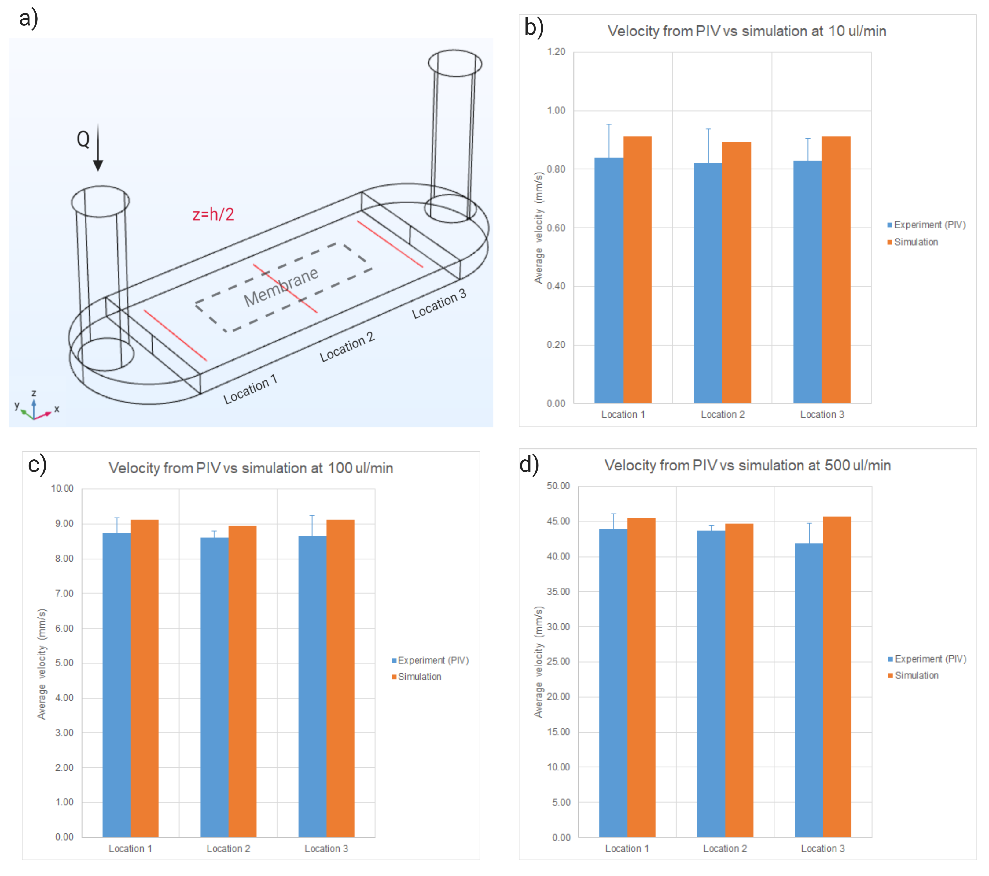
Fig. 2. a) Schematic of the flow module. Dash lines show the location of the membrane which lies below the flow module (Red lines show locations at which velocities from PIV and simulation have been obtained and compared; these lines are located at the middle plane of the channel: z=h/2). Comparison of velocities obtained from PIV and simulation at a flow rate of b) 10 ul/min, c) 100 ul/min, d) 500 ul/min. (error bars represent one STD).

3.2. Shear stress 

As shown in Fig. 3, the flow is fully developed as it reaches the membrane. Also, the shear stress is uniform at the membrane surface (Fig. 4).

Fig. 3. Velocity magnitude along the channel length (The red line is located at y=w/2 and z=h/2).

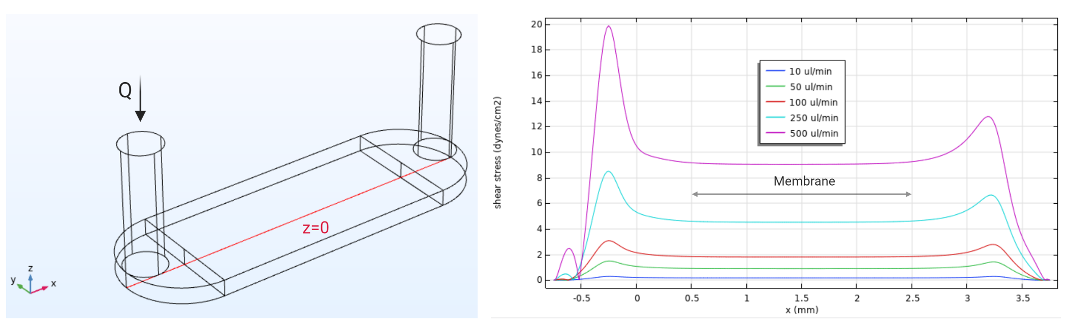
Fig. 4. Shear stress magnitude along the channel length (The red line is located at y=w/2 and  z=0).

The maximum shear stress within the module occurs at the intersection corner of the channel and outlet as shown in Fig. 5.

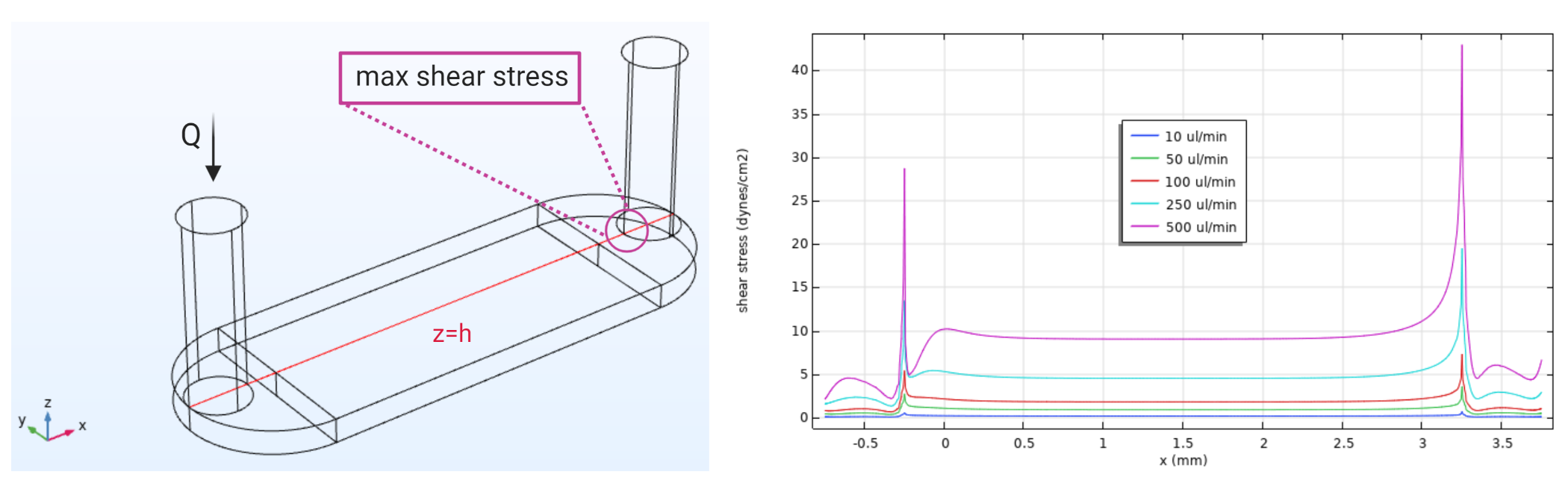
Fig. 5. Maximum shear stress magnitude within the flow module (The red line is located at y=w/2 and z=h).

In Table. 1, corresponding shear stress at the membrane surface and maximum shear stress within the device are reported for different flow rates.

Table. 1. Flow rate selection guideline based on the required shear stress

Update (Feb 5, 2021)

The velocity profile along the width and height of the channel is shown in Fig. 6.

Fig. 6.  a) Channel width (y), b) channel height (z), c) velocity profile along the y-axis, d) velocity profile along the z-axis.