Nano-pocket Membrane Pressure Modeling
Introduction:
In the previous post, we demonstrated our capability to fabricate the nano-pocket membrane and effectively capture and release particles of various sizes. In this post, our focus shifts to exploring the membrane capability. We will focus on the membrane modeling (parking point, the plateau region)of the nano-pocket membrane.
To have an overview of the membrane, the final nano-pocket membrane shape has been fabricated has a wide opening (500-700 nm) on top that narrows down to a smaller opening on the bottom side (150 to 250 nm), with a thickness in a range of 1.5 to 2.5 µm (figure 1).
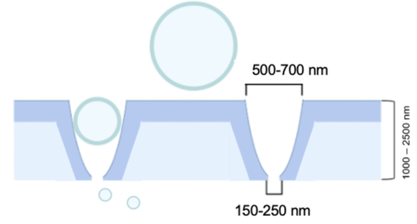
This illustration shows the final membrane shape. It indicates that the top pore size is larger than the bottom pore size, and that the membrane’s thickness depends on the photoresist thickness (represented by light blue) and the amount of parylene on top (represented by dark blue).
Tangential Flow for Analyte Capture (TFAC) Device Design:
Figure 2 shows the various layers of the microfluidic device. At the top, a 3D-printed component features chambers thoughtfully designed to accommodate standard microfluidic tubing connectors. These chambers form a seamless connection with the succeeding components, two precisely aligned adhesive layers, with a nano-pocket membrane expertly ensconced between them. To ensure the device’s integrity and to prevent any potential leakage, a cover glass is meticulously affixed at the bottommost layer. This layers results in the successful creation of the fully assembled microfluidic device, as depicted in figure 2b. Furthermore, the orientation of the membrane’s larger opening facing downward, as depicted in figure 2c, is of paramount importance. Finally, the numerical designations assigned to ports b and c underscore their identical functionality, serving as both the inlet and outlet for the device.
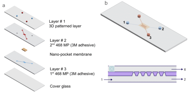
a) Starting from the top, a 3D-printed part includes chambers designed explicitly for standard microfluidic tubing connectors. Next, there are two aligned adhesive layers with a nano-pocket membrane sandwiched between them. Finally, a cover glass is placed on the bottom to prevent any potential leaking and provide additional protection to the device. b) The image depicts the final assembled device. c) The membrane’s larger opening is facing downwards. The numbers in panels b and c represent the same inlets and outlets on the device.
Experiments and Results:
Prior to employing the membrane device, the pressure caused by tubes was examined. Each tube has an inside diameter of 0.01 inches and a length of 15 inches. In the first experiment, only one tube was utilized. The setup sequence consisted of a pump, followed by the tube (T1), and finally, a pressure sensor (P1). For the second experiment, an additional tube and pressure sensor were introduced. The setup sequence entailed a pump, followed by tube #1 (T1), pressure sensor #1 (P1), tube #2 (T2), and pressure sensor #2 (P2). Lastly, the final tube and pressure sensor were incorporated into the setup after P2.
Figure 3 illustrates the pressure caused by the tubes. The experimental setup is depicted in (a). For the first experiment, the pump was connected to the T1, which was connected to P1. In the second experiment, a new tube with a new sensor was added. Similarly, in the third experiment, a third tube and sensor were added. The pump flow rate was approximately 20 µl/min. The results indicate that the tube has an effect at this flow rate. In the first experiment, there was no pressure difference, while in the second and third experiments, the tube exhibited a pressure effect of 0.2 PSI.
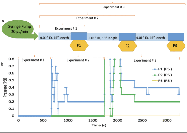
a) Experiment Setup: This panel illustrates the experimental setup, showing the pump connected to a number of tubes and sensors (P1, P2 and P3). b) Experiment Results: This panel presents the results of the three experiments conducted: 1) Just P1 from 0 to approximately 600 seconds, indicating a pressure of 0 PSI. 2) From 600 to approximately 1700 seconds, displaying pressures of 0.2 PSI for P1 and 0 PSI for P2. 3)The addition of P3, with pressures of 0.4 PSI for P1, 0.2 PSI for P2, and 0 PSI for P3, respectively, as observed results.
Afterward, we investigated the effect of a T valve as a control for the experiment. The T valve provided the ability to regulate the flow from valve #1 (V1) to either valve #2 (V2) or valve #3 (V3). The experimental setup is illustrated in Figure 4a. In the first experiment (with V3 closed), the flow proceeded from the pump to P2. It passed through T1, V1, and P1 to reach T2, V2, and finally P2. In the second experiment (with V2 closed), after passing through T1 and V1, the flow was directed to T3, V3, and P3.The results revealed a consistent pattern observed in the previous experiment. Initially, P2 exhibited fluctuations before stabilizing at 0.2 PSI. These findings indicate that the tube exerts a 0.2 PSI effect on the pressure sensors, consistent with our earlier observations.
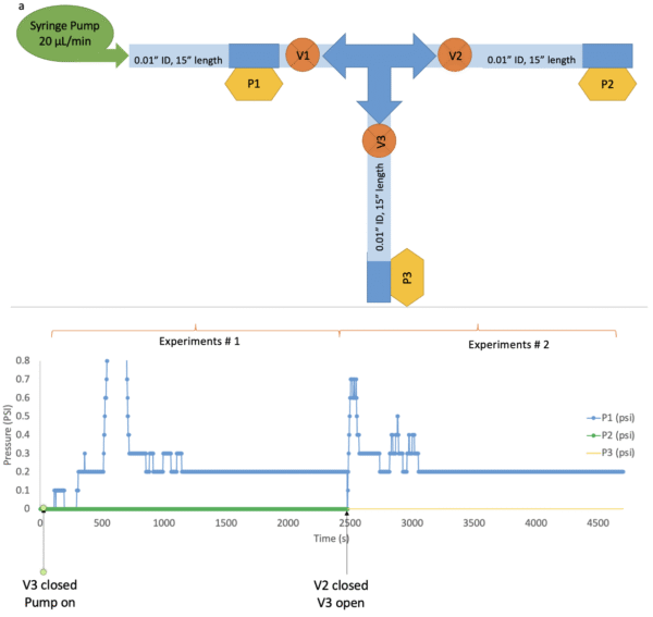
a) Experiment Setup: This panel illustrates the experimental setup, depicting the pump connected to a T valve and sensors (P1, P2, and P3). b) Experiment Results: This panel presents the results of the two experiments conducted: 1)P1 from 0 to approximately 2500 seconds, indicating a pressure of 0.2 PSI. 2) From 2500 to approximately 2700 seconds, displaying pressures of 0.2 PSI for P1.
Device with a membrane experiments:
Subsequently, we examined the pressure using a nano-pocket membrane. Initially, our focus was on analyzing the flow in the bottom channel, where the fluid does not pass through the membrane (figure 5 a). Our findings revealed that the pressure reached 0.3 PSI. It is noteworthy that the initial P1 measurement before commencing the experiment was recorded at 0.1 PSI (figure 5 b).
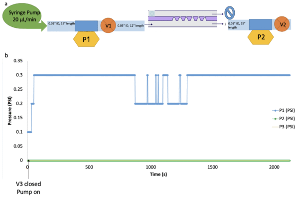
a) Experiment Setup: This panel illustrates the experimental setup, depicting the pump connected to a nano-pocket device. The flow is just on the bottom channel. b) Experiment Results: This panel presents the results of the bottom channel being open (where the flow does NOT pass through the membrane). P1 is plotted from 0 to approximately 2200 seconds, indicating a pressure of 0.3 PSI. Before starting the experiment, the pressure was measured at 0.1 PSI.
Dead-end mode:
The next step is to study the pressure in dead-end mode. The flow passes through the nano-pocket membrane to reach the top channel and exit the device (see Figure #6a). The results indicate a plateau region where pores begin to be blocked by particles in the fluid (see Figure #6b). Subsequently, the pressure increases due to pores becoming clogged by the particles. The failure point, marking the point at which the membrane structure fails or breaks down under the applied pressure, occurs between 16500 and 1900 seconds.
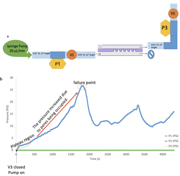
a) Experiment Setup: This panel illustrates the experimental setup, depicting the pump connected to a nano-pocket device. The flow is passed through the membrane. b) Experiment Results: This panel presents the results of the flow being passed through the membrane open. P1 is plotted from 0 to approximately 4000 seconds, indicating a pressure is increasing until it reaches the failure point around 1700 seconds. The membrane was broken at around 25 PSI.
In this experiment, it’s assumed that 40% of the pores are occupied suing Dagan equation. The Dagan equation, which calculates pore resistance, is expressed as:
![]()
Where:
- represents fluid viscosity (0.001 Pa s),
- denotes the pore radius (7.50E-08 m or 75 nm),
- signifies the pore length (1.50E-06 m or 1500 nm).
Using the given values, the calculated pore resistance is 1.28E+20. However, to determine the total membrane resistance , we sum the resistance for each pore in parallel, totaling 4.29E+05 pores.
The pressure drop can then be calculated using the formula:
Where represents the flow rate (2 µl/min), and denotes the total resistance (2.98E+14).
The resulting pressure drop is 14.4 PSI.
When 40% of the pores are occupied, the pressure drop is observed to be 24.02 PSI, matching the experimental findings.