Matlab Generated Endothelial Cell Alignment Distribution
Top and Bottom Gel
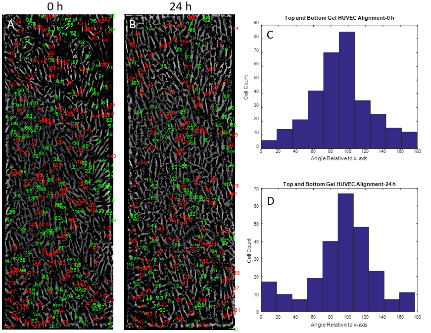
Figure 1. Matlab based alignment semi-quantification of HUVECs seeded on top of a collagen I gel. (A) Matlab output of major axis angle (relative to the x-axis) of HUVECs before flow set on top of cell image. (B) HUVEC angle of alignment relative to x-axis after 24 h flow. (C) Histogram plot of A, angles changed to reflect y-axis alignment. (D) Histogram plot of B.
No Gel
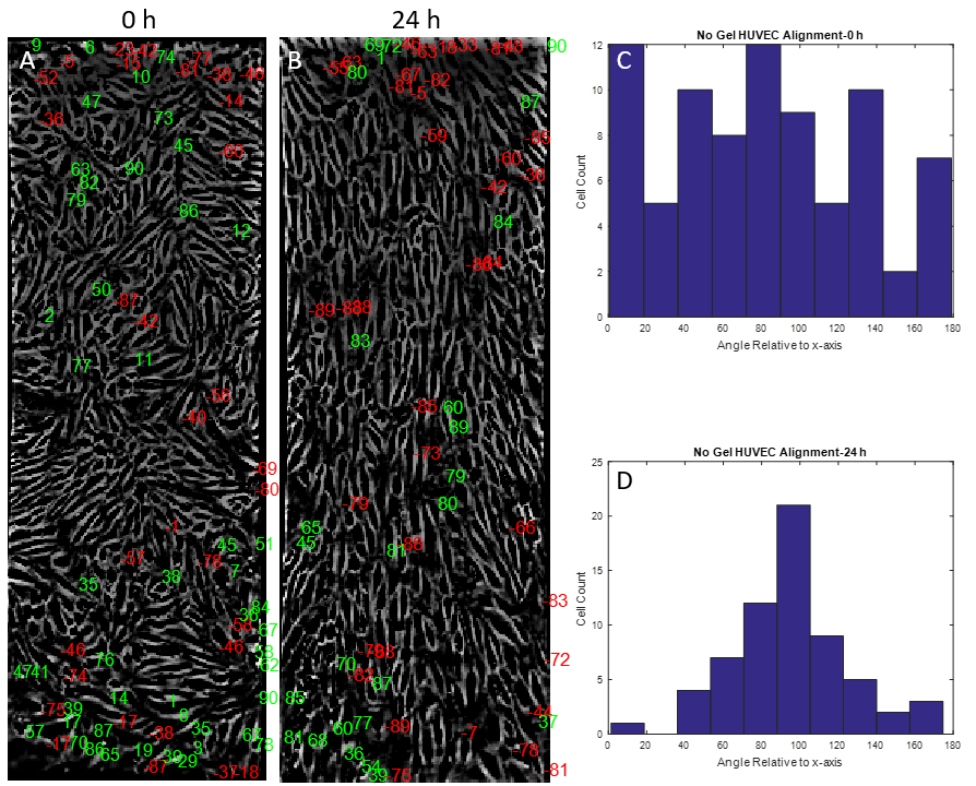
Figure 2. Matlab based alignment semi-quantification of HUVECs seeded directly on the NPN chip. (A) Matlab output of major axis angle (relative to the x-axis) of HUVECs before flow set on top of cell image. (B) HUVEC angle of alignment relative to x-axis after 24 h flow. (C) Histogram plot of A, angles changed to reflect y-axis alignment. (D) Histogram plot of B.
Bottom Gel
Run 1
Figure 3. Matlab based alignment semi-quantification of HUVECs seeded directly on the NPN chip with collagen I gel on the reverse side. (A) Matlab output of major axis angle (relative to the x-axis) of HUVECs before flow set on top of cell image. (B) HUVEC angle of alignment relative to x-axis after 24 h flow. (C) Histogram plot of A, angles changed to reflect y-axis alignment. (D) Histogram plot of B.
Run 2
Figure 4. Matlab based alignment semi-quantification of HUVECs seeded directly on the NPN chip with collagen I gel on the reverse side (RUN 2). (A) Matlab output of major axis angle (relative to the x-axis) of HUVECs before flow set on top of cell image. (B) HUVEC angle of alignment relative to x-axis after 24 h flow. (C) Histogram plot of A, angles changed to reflect y-axis alignment. (D) Histogram plot of B.
Statistical Analysis
The next step in this data analysis is to perform some form of statistical analysis. Comparing real alignment data to a set of randomly generated alignments may be a good place to start. Also, comparing the frequency distributions of the before flow and after flow alignment histograms may provide some level of significance.
Example Shear Calculations with 1um Polystyrene Beads
Matlab Video Processing
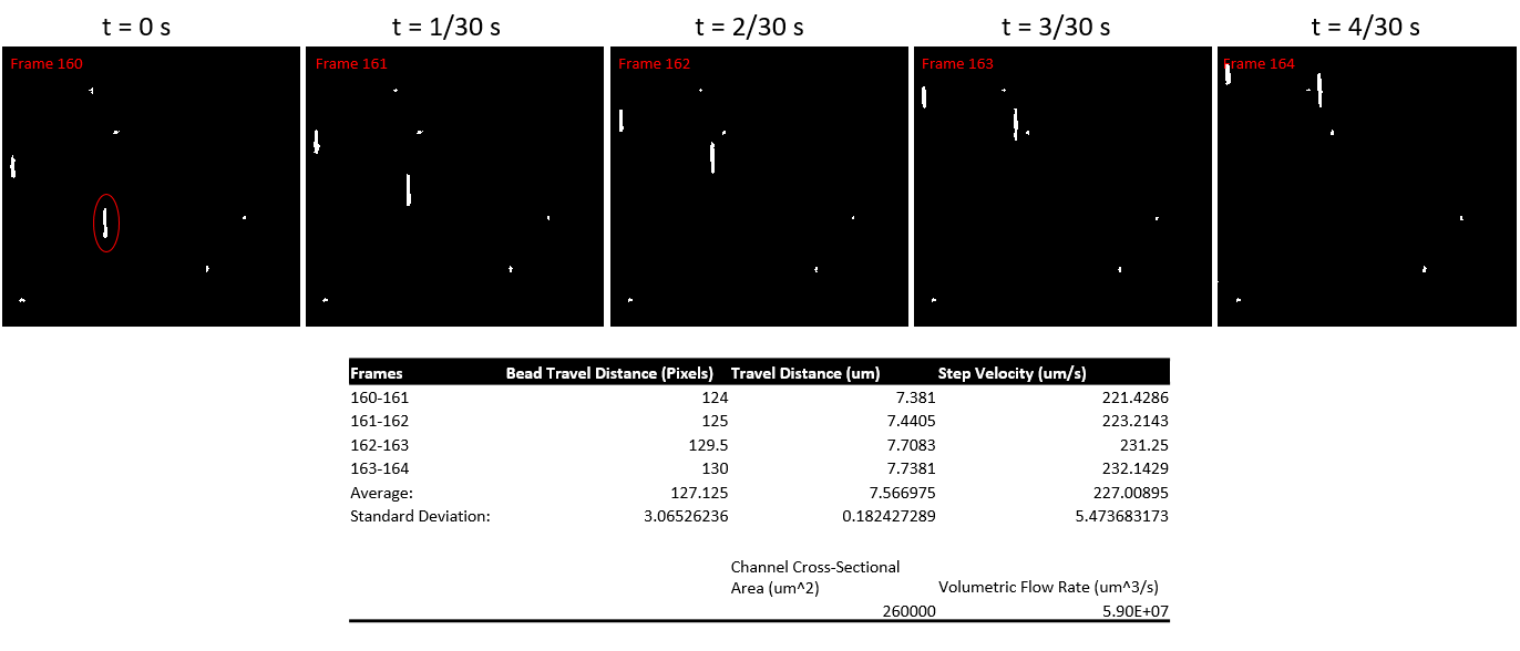
Using matlab, the video seen above was converted to gray scale frames, which were then converted to binary images (Figure 5). Matlab then tracks the center of the particle over 5 frames and calculates a distance traveled in pixels, distance traveled in um, and velocity in um/s.
Figure 5. (Top) Images showing particle trajectory over 4/30 s. Each picture represents a frame of a video shot at 30 fps. The particle circled in red was used to obtain velocity. (Bottom) Data from matlab analysis on particle velocity.
Using the formula for shear flow through a slit:
τ=6Qμ/(wh^2 )
I calculated a shear at the surface of the gel of about 0.093 dyn/cm^2. The expected shear at this level is around 6.5 dyn/cm^2.
In this post I address every objective we started with and summarize our results: a) Building of research capacity at Fisher. —–> We would like to to produce our lipid-based nano particles in a cheaper and more reproducible way. For the last 4 weeks Ryan has been producing phosphatidylcholine liposomes. Depending on the rate of flow, we…
Vaccinex has developed an antibody, VX15/2503, for Semaphorin 4D, a molecule implicated in axonal guidance mediation and blood brain barrier (BBB) disruption. The role of SiMPore in its partnership with Vaccinex is to produce a workable model of the BBB, with the ability to introduce flow conditions and measure an electric gradient across the membrane. …
Recently, I have been trying to pass 5 nm, 10 nm, and 15 nm gold through untreated, carbonized, and ozone/carbonized membranes. These experiments were done in the pressure cell with fresh samples. I used a 1:1 dilution of Au stock and DI water. To wet the membrane I placed a 40 uL drop of water…
I got some wafers from Chris last week(?) that had undergone different Megasonics cleaning treatments by the manufacturer. We’re trying to figure out if these treatments are actually cleaning the wafers. I’ve been having trouble getting the AFM to stay in the “right” mode for imaging with these wafers. However, I have gotten some images….
The question arose last week about the affects of transport with use of the shaker in the Tecan, which led to a discussion about the current construction of the sepcon. The sepcon layout currently is as follows: The o-ring is 1 mm in diameter. Is this difference between the membrane and the receiver fluid dead…
Here is the paper I reviewed at the NRG meeting on 06/19. Utah Group Micro BBB Device I’ve also included my presentation: BBB Device Presentation This week I’m working on designing the basal and apical chambers, considering the necessary shear stresses.