Theoretical Underpinnings of Small Molecule Permeability Measurements in the µSiM (Part 2: Experimental Validation)

This is the second installment in a series of posts focused on the development of a method for measuring barrier permeability in the µSiM. In Part 1 we discussed the goal of making these measurements in situ at a position beneath the membrane. Because our preference is to use the trench down configuration in the R61 studies, this means that the measurement is to be made inside the trench (recall that chips are 300 µm thick). We also saw that COMSOL simulations of diffusion in our device indicated that a simple 1D analytical model of diffusion would be appropriate for interpreting these measurements – assuming we can make them.

In this post we present experimental evidence that confocal imaging 100 µm beneath the membrane looks the right approach for in situ permeability measurements. All experiments shown here use 1 mg/mL 10kDa dextran-AF488.

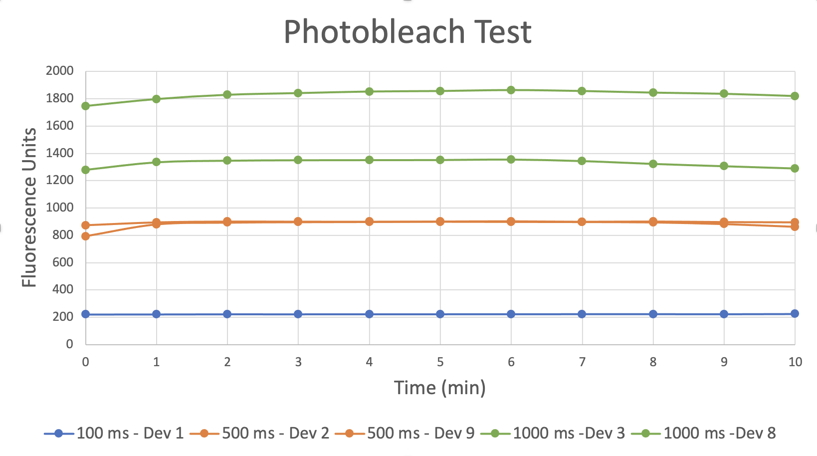
This test shows measurements 100 µm below the membrane taken with different exposures with both top and bottom channels flooded with dextran-AF488. We never see evidence of photobleaching even with exposures of 1 s. We switched to AF488 because it is more photostable (and less pH sensitive) than FITC. However, Molly has also found that FITC does not bleach appreciably over 10 minutes with 1s exposures taken every minute, so that data may appear sometime in a later post.

Next we show a sequence of images that shows that we get a diffusive time series of images when we added dextran-AF488 to the top well and focus the spinning disk confocal focused 100 µm directly below the membrane:

That this works is demonstration of the power of confocal microsocopy. We can appreciate with a direct comparison to a widefield experiment that was otherwise done the exact same way:

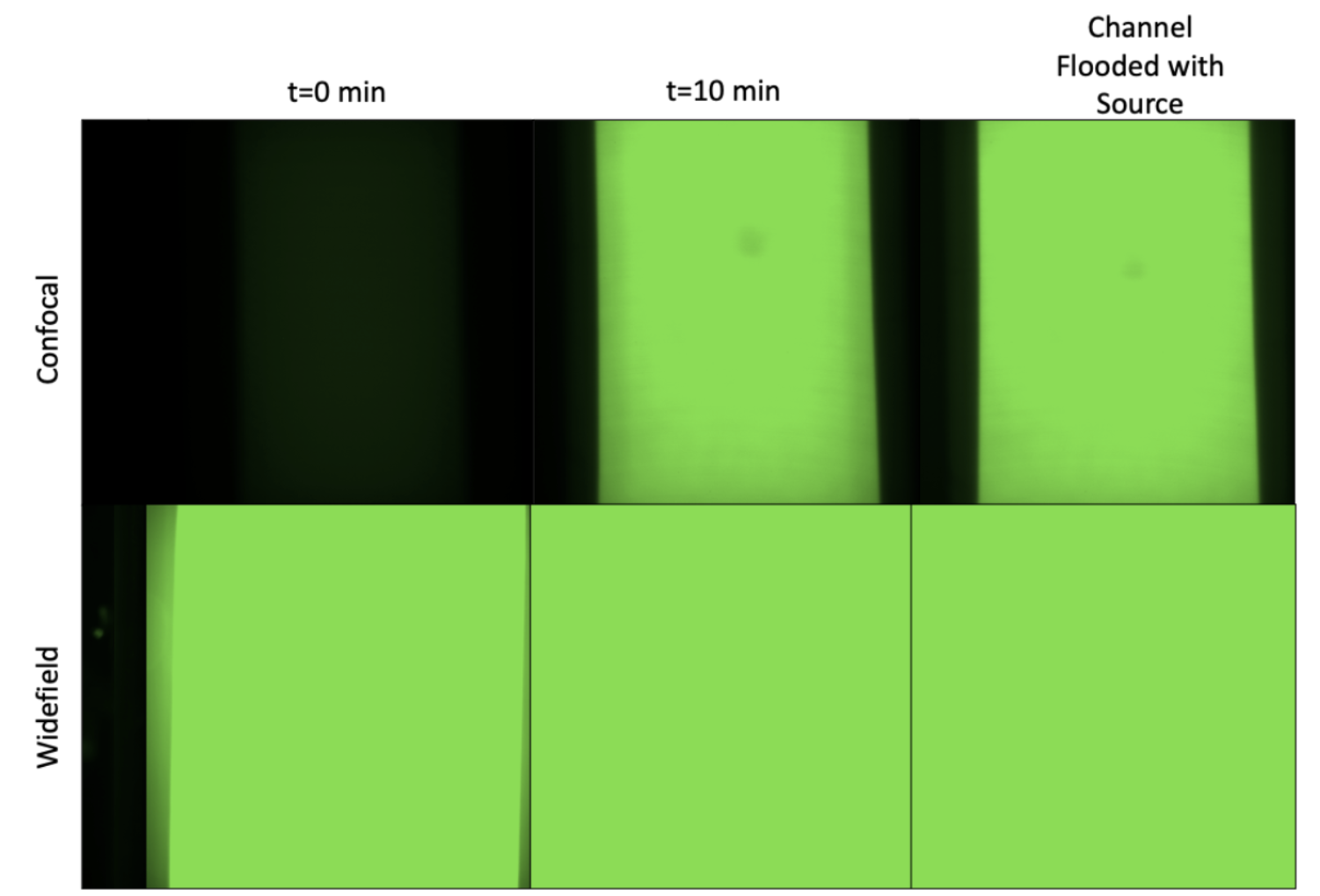
So in widefield microscopy, the well contributes an overwhelming amount of out-of-plane fluorescence when measurements are taken 100 µm below the membrane. The camera and we cannot is saturated from the start.

Molly has also done an experiment to justify the choice of imaging 100 µm below the membrane. The experiment used a non-porous membrane with the well loaded with dye and took consecutive slices from the membrane to a position 250 µm below: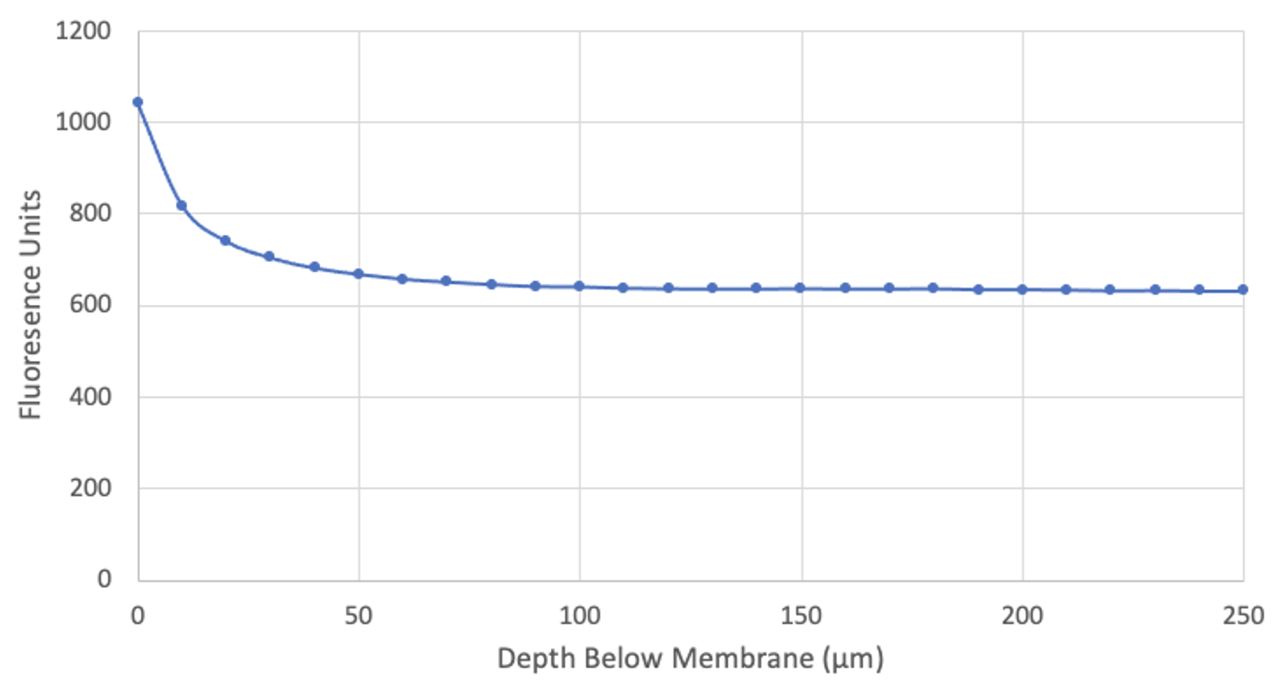

This is the corresponding movie. It actually plays backwards, so it starts in the trench and inches forward to the membrane. Note that only when the membrane comes into focus does the fluorescence begin to increase.

So beyond ~100 µm the well fluorescence gives a minimum background that no longer sensitive to position. Anyone setting up their experiments elsewhere should do this same study to make avoid experiment-to-experiment variation in the backgound. Please note that while we used our Piezo stage to drop the objective 100 µm physically, due to the air-water interface, the focal plane actually drops ~133 µm (for explanation, see here).

[Why is there a background where  because there is no dye in trench or bottom channel?  While there is minimal collection of out-of-plane light by our objective due to the confocal nature of our imaging, there is still a transmission of light into the trench space and reflections of light off the trench walls. This light must reach the plane of imaging. Kinda like turning on a lamp in the corner of an otherwise darkened room?]

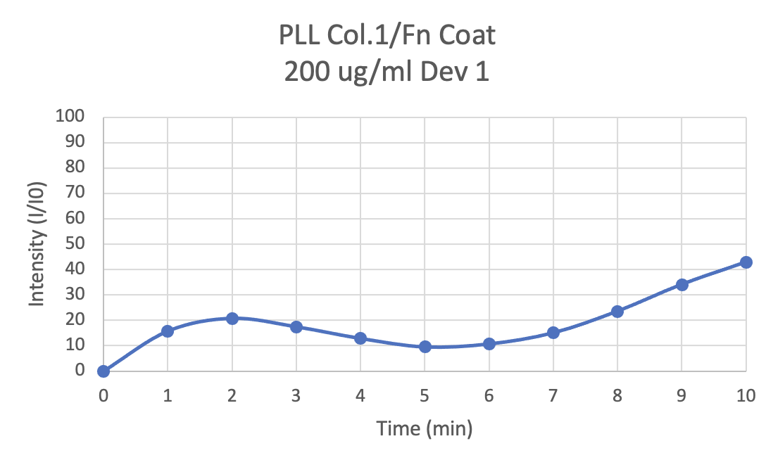
The final step for the validation of our method is to make a measurement of diffusion and show that the 1D analytical model can explain the measurement. We did this by introducing 10 kDa dextran-Alexa 488 to the well and monitoring the fluorescence at 100 µm using 1s exposures every minute for 10 minutes. We found it was necessary to replace the entire 100 µL well volume because when we replaced only 50 µL (adding to an existing 50 µL without dye) we saw a fluorescence ‘wave’ that we associated with the incomplete mixing of the dye. The image below is typical of what happens in this case:

The approach of replacing the entire top well volume would not be desirable with cells. Fortunately we have found we do not get this wave with cells because of the longer transport times (Cell protocols to come in Part 3).

Recall from Part 1 that the 1D diffusion equation that matched our COMSOL simulations nicely was:

If we change from concentration to fluorescence and include the effects of a background fluorescence we get the equation to fit to our data:

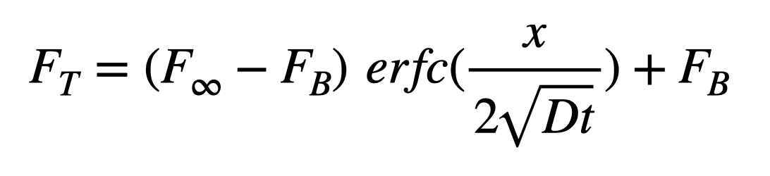
Here F_T is the total fluorescence F_∞ is the final fluorescence and F_B is the background fluorescence. D and t are the molecular diffusion coefficient and time, respectively, and x is the location of the concentration measurement away from the inexhaustible source (x = 100 µm…This was used in early iterations before we were aware of the “fishtank effect“, now x = 133 µm).

[Fluorescence is not equivalent to concentration. The presence of  background in a fluorescence measurement is one way these are different, but if account for the background we are only assuming they are proportional to each other. Concentration-based quenching of fluorescence signal can challenge this assumption but Molly has also checked that we are working in a linear regime in these experiments (Molly is thorough!)].

Now we have three unknown parameters in the above equation F_∞, F_B, and D. We can fit all three of these or try to independently measure F_∞ and F_B and fit only to D. It is best to use as few free parameters as possible, so we explored one, two and three parameter fits. We used the initial measurement (t = 0) as the background F_B, and flooded the backside of the device with media from the well after the experiment to get an estimate of F_∞. This is Molly’s modification of the method originally developed by Alec (Khire et al. 2000). Here are the results:

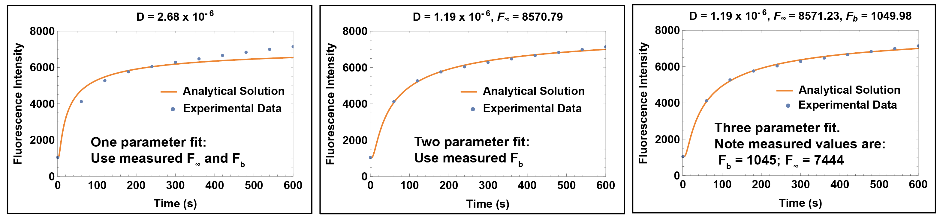
The one parameter fit clearly doesn’t work. It rises too fast at early times and not fast enough at later times. Both the two parameter and three parameter fits give curves that match the dynamics of the data very well. This suggests that we have the physics right, which is a big step. The fact that we need at least a free second parameter means that we really don’t know either F_∞ or F_B despite our attempt to measure these. Because the two parameter fit uses the measured F_b and the three parameter fit actually predicts our measured F_b, it is clear that F_∞ is the culprit parameter. For some reason we can’t quite trust the value we get by flooding the backside of the device with the well solution.

It seems the best approach is to let the curve fit find F_∞ and use our measured F_b from the t = 0 measurement. This simplifies the experimental protocol, which is a bonus.

The second thing to notice is that the predicted value for D in these experiments is spot on according to Shoga et al, Annals of Biomedical Engineering 45, 2461–2474(2017) who used fluorescence correlation spectroscopy (FCS) to measure the free diffusion coefficient of 10kDa dextran-Alexa488.

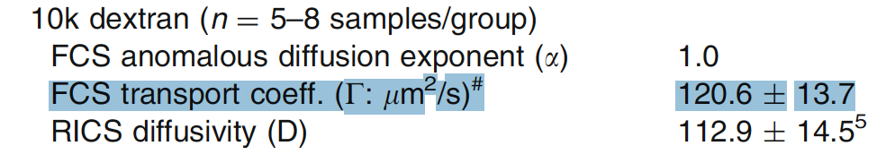
When we repeated this measurement we ended up with a slightly lower mean (0.92 ± 0.14) for a set of three experiments, but I don’t think there is a statistical difference between our results and Shoga’s. Since FCS is a measure of molecular self-diffusion in a volume, I take this as more evidence that the membranes are so permeable that they do not hinder small molecule diffusion.

Update (4/16/21):  We repeated the above analysis for our coatings and found that the coatings did hinder tracer diffusion compared to uncoated NPN. We checked both the PLL/Col1-Fn coatings that we use for pericyte/EC co-culture, and the Col1-Fn coating that we use for ECs. We were a little short on statistical power with the PLL/Col1-Fn set but the Col1-Fn showed a statistically significant reduction (p < 0.05) of more than a 50% for 10 kDa Alexa488-dextran.

These diffusion coefficients very likely mean we can ignore the need to subtract the ‘system permeability’ as is conventionally done with transwells. We’ll examine this a bit more closely in Part 3 but as a preview, even with the coatings the ‘system permeability’ comes out to ~ 0.014 cm/min which is multiple orders of magnitude higher than we expect to see for EC barriers.