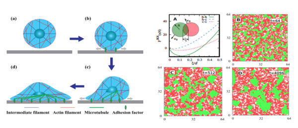
Cell-substrate interaction modeling
The idea of this project started when we were writing a mini-review about cell-substrate interaction. Although most of studies of cellular responses to porous membranes have pointed towards a multiphasic response with the same trend of changes with respect to the pore sizes, we also found some variation in the results. We suggested that some of the variations in published results are likely due to the use of different cell types, substrate materials, and experimental methods. Since experimentally testing the effect of all variables, including cell and substrate properties, on various cellular behaviors is costly and time-consuming, computational modeling may be an effective approach either as an alternative for these experiments or for confirming and extrapolating the results from them.
Computational modeling is already used for understanding some cell-material interactions. Some of the developed models recapitulate single cell response to an environment, while others simulate collective behavior of cells. Similar approaches with small adjustments can be employed for analyzing interactions of different cell types with varying abilities for generating traction forces over porous membranes of different mechanical and physical properties. The main modification, which is required for these models to be applicable for porous membranes, is to define the pores in their equations.
Since we were going to study cell migration, we decided to use the second latter approach for our project. After consulting with Dr. Das, we chose the self-propelled Brownian particle approach and consider the membranes as a potential field in the model.
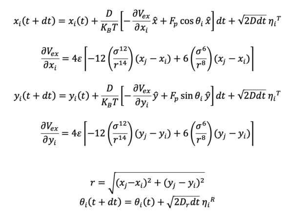
In the model that we started with, each cell is self-propelled with a constant force, and interactions between cells result from isotropic repulsion. Here is the related equation:

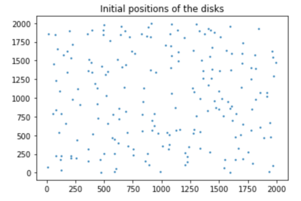
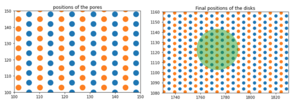
Initial configuration
We first needed an initial configuration. We needed a 2D system consisting of N identical disks of diameter sigma. We determined a square simulation box (where the whole cells are) of size L. We also make sure that the centers of no two particles are closer than a specified distance. This means that our initial configuration builder allowed for overlaps between particles to a specific extent. The code defines the random position of the cells one by one to avoid the full overlap.
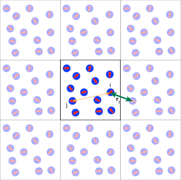
In our system, the instantaneous position of cell i is given by the vector r=xi+yj. In addition, each disk is polar and its polarity is described by a vector theta, where is the angle between and its direction and the axis X. The etha(T) and etha(R) are translational and rotational Gaussian white noise variables. Here is our equation:
- Since the derivative of potential should be calculated between every two cells, we need to define neighbors to make the calculation faster.

Fig.3. Neighboring condition in the code. - We also needed a boundary condition to contain the cells (like the sample walls).
- We had two choices for the walls, periodic boundary or fixed boundary.
- We decided to choose a fixed boundary because of the number of our cells.
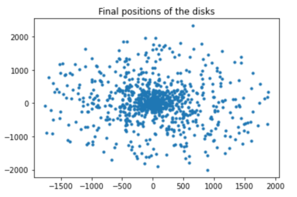
We finally achieved our model based on the self-propelled Brownian particle approach without considering the membranes.
The next step was to determine a parameter that could replicate our membranes. We had two choices:
- Adding it to the self-propulsion force
- Defining it as a separate parameter
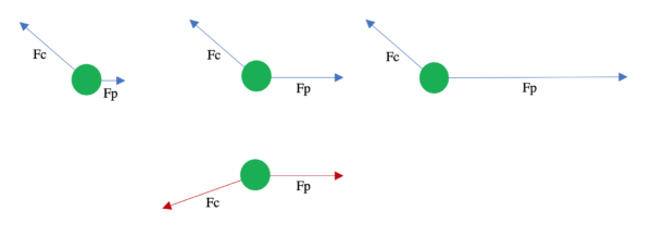
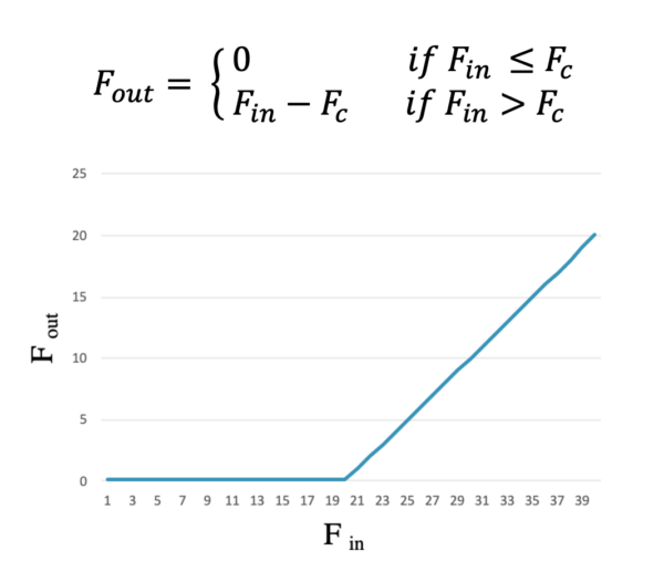
Since we need an independent parameter for this interaction, we suggested a piecewise function for it:
Having two separate parameters for cell-substrate adhesion and traction forces can better explain the biphasic relationship between speed of migration and substrate stiffness.

After having the main code for the cells with the membrane component, we developed the code for the membranes.
In the first step, we considered the pores as the areas that should be subtracted from the whole cell area. So, the number of pores and their area (overall porosity) is the only important factor in the calculation.
I ran the code and compared the results with the experimental data. As you can see, there is not much difference between 3-micron and 0.5-micron pores. But considering that the mentioned condition just can resemble the pore opening, we need a parameter for the pore edges (we previously predicted that may serve as gripping sites, or at least provide more adhesion areas)

The next step was adding a parameter for the pore edges. We decided that it would be more meaning full to be added to the self-propulsion force because it also should be in the direction of the traction forces. Adding this new parameter increased the speed of migration for 3-micron pore membranes. I did not run the code for the 0.5-micron yet.
Another approach for adding the pores to the main code is to considered them based on their position with respect to each cell. In this approach the distance of pores from the center of the cell, instead of their number, is important. I am working on this approach as well to compare the result with the previous approach and experimental data.

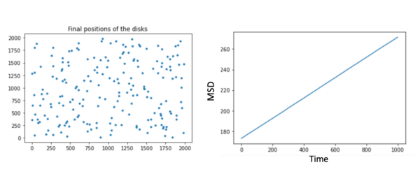
For very long times your MSD vs. time plots should flatten at the size of your bounding box (squared).