shear stress reduction via pnc-Si: COMSOL simulation
Hi all! Last time we have presented a theoretical perspective on the shear stress reduction enabled by our shear-free microfluidic system. This time we will show an agreement between the shear-reduction predictions made by the analytical solution and a COMSOL simulation. For details on the analytical solution please refer to the following post: [https://trace-bmps.org/datablog/2012/04/26/shear-stress-reduction-via-pnc-si-analytical-solution/]
COMSOL Simulation:
Due to the large difference in the order of magnitude of dimensions (at least 10^7 fold) between the pore and the flow compartment, it is impractical to perform FE method pore-by-pore. We have therefore resort to modeling the membrane as a porous media using the Brinkman’s equation. The Brinkman’s equation requires that we know the porosity and the permeability of the membrane. The permeability of a porous media is defined by k = (v)(u)(dx/dp), where k is the permeability, v is the fluid velocity, u is the fluid viscosity, dx is the distance the fluid traveled (aka membrane thickness), and dp is the pressure drop. Luckily, we can calculate the permeability from Jirachai’s EO data [https://trace-bmps.org/wp-content/uploads/2011/09/EO_Testing_Report.pdf].
i arbitrarily chose the case in which no voltage is applied, dp = 0.2 psi (1378 Pa), and the flow rate is ~ 400 nL/min to get a general estimate for the permeability:
(400nL/min)/(2x 2000um*100um)(1 mPa*sec)(15 nm)/1378 Pa = 1.81*10^-19 m^2
Since only the volumetric flow rate is given, we have to obtain the velocity through division by the total membrane area. I was told that each membrane area of the 2-slit chip that Jirachai used is 2000 by 100 um. I do not know the porosity of the membrane that Jirachai used but I will use the value of 10% to match the analytical solution.
Below is an example of the COMSOL simulation:
geometry:
top chamber (flow compartment): length = 2.5 mm, height = 200 um
middle layer (membrane): membrane thickness = 25 mm
bottom chamber (shear-free compartment): length = 2.5 mm, height = 100 um
material properties:
membrane/porous media properties: porosity = 10%, permeability = 1*10^-15 m^2
water: density = 10^3 kg/m^3, viscosity = 10^-3 Pa*sec
boundary conditions:
inlet flow velocity = 1 um/sec, outlet pressure = 0 Pa, no slip condition everywhere else.
Figure 1 below shows the COMSOL FE analysis results, with the flow velocity in the shear-free compartment as a function of the system length plotted (which is parabolic). The red line in the shear-free compartment highlights the path of the line scan of flow velocity.
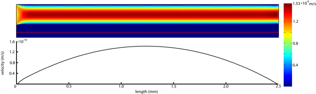
Unfortunately even after the simplification with the use of the porous media we still cannot get down to the membrane thickness of 15 nm. However, we noticed that the maximum velocity seen in the shear-free compartment is directly proportional to the membrane thickness. While the maximum velocity seen in the shear-free compartment is not linearly proportional to permeability, we can extrapolate the maximum velocity by taking the regression of the maximum velocity as a function of a 4th order polynomial of the permeability. Base on the above methods, a membrane 15nm in thickness and a permeability of 1.81*10^-19 m^2 yielded a maximum flow velocity of 1.97*10^-10 m/s.
Analytical Solution:
We will use the following values to approximate our shear-free microfluidic system (the same specs as the hybrid membrane that i used for my shear-free chemotaxis chamber):
porosity = 10% [ ratio of the distance of the pore to that of “non-pore” = sqrt(0.1) ~ 0.31 ]
for R1: r1 = 15 nm (pore diameter of 30nm) and l1 = 12.5 um (membrane thickness).
for R2: l2 = length of non-pore + diameter of pore (~95 nm), w2 = l2, h2 = 200um.
for R3: l3 = length of non-pore + diameter of pore (~95 nm), w3 = l3, h3 = 100um.
the length of the shear-free microfluidic system will be 2.5mm (26352 repeats of circuit loop).
input flow velocity: 1*10^-6 m/s (1um/sec)
RESULT: max velocity at the shear-free compartment = 1.72*10^-10 m/s (compare to 1.97*10^-10 m/s from COMSOL simulation).