Incorporating Concentration Polarization into Our Convective Sieving Model
Prior to my qualifying exam about a month ago, I put together a simple model of transport (detailed in this previous post) across a nanomembrane that incorporated electrostatics as well as terms describing both convective and diffusive transport across the membrane. It was a useful model, but ultimately limited, as shown by the following image:
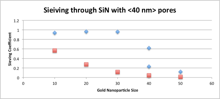
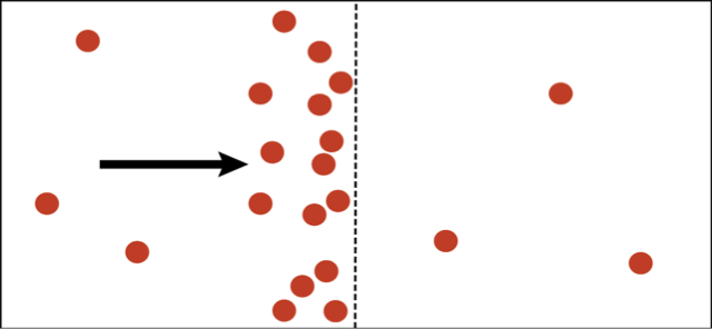
This graph shows predicted sieving coefficients (red) for a size ladder of gold nanoparticles using actual pore distributions, as compared to experimental results (blue) for the same membranes. Note that experimentally we get the really sharp cutoffs we’ve come to expect from pnc-Si and SiN membranes, but the model utterly fails to capture this behavior. I believed that the reason the model was failing was the fact that it had failed to account for the fact that the local concentration of gold at the membrane is higher than in the feed, as shown below:
After speaking with our Clarkson collaborator Ruth Baltus and scouring the literature, I’m more convinced than ever that if we want our model to show sharp cutoffs, we will need to account for this localized concentration increase, which is also referred to as concentration polarization.
As justification, recall that our model was based on the following set of equations:


![\langle N \rangle = W\langle V \rangle C_{\text{feed}} \frac{[1-(C_{\text{filtrate}}/C_{\text{feed}})e^{-Pe}]}{1-e^{-Pe}} \ \ \ \ (4)](https://s0.wp.com/latex.php?latex=%5Clangle+N+%5Crangle+%3D+W%5Clangle+V+%5Crangle+C_%7B%5Ctext%7Bfeed%7D%7D+%5Cfrac%7B%5B1-%28C_%7B%5Ctext%7Bfiltrate%7D%7D%2FC_%7B%5Ctext%7Bfeed%7D%7D%29e%5E%7B-Pe%7D%5D%7D%7B1-e%5E%7B-Pe%7D%7D+%5C+%5C+%5C+%5C+%284%29&bg=ffffff&fg=000&s=0&c=20201002)
where 


To calculate the filtrate concentration of gold (which we need to calculate the diffusive flux) , we assumed that there was no concentration polarization and that the system was in steady state. In essence, we claimed that once gold is ‘rejected’ by the pore it ‘disappears’ forever (ignore for the moment that this violates the conservation of mass). This rejection of gold is defined by the rejection coefficient 
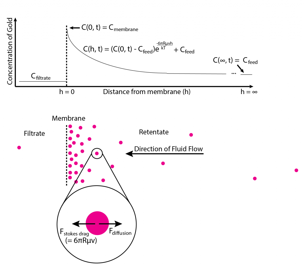
If instead of instantaneously disappearing after being rejected, the gold hangs around the entrance and only slowly diffuses back into the bulk (i.e. if we account for concentration polarization), the localized increase in gold concentration serves to increase both the diffusive and convective flux (of gold) across the membrane.
There’s experimental evidence that seems to back this up, too. Even with thicker membranes, the following paper found that solute flux across a membrane increases both when the filtration cell was unstirred and when the pressure drop across the membrane increases, a result that they attributed to the associated rise in concentration polarization in both cases: (Ultrafiltration of gold and latex, S.S. Madaeni). This paper (link to abstract, we don’t have access yet) similarly found that not stirring in dead-end filtration increases gold flux across a membrane.
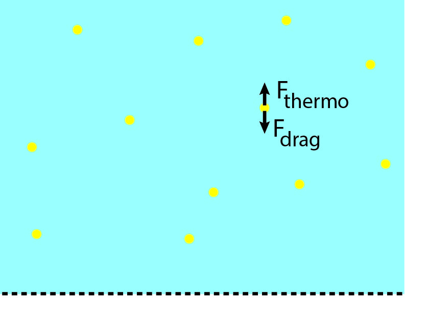
The first thing to recognize is that the gold particles at the membrane are acted on primarily by two forces – a stokes drag exerted by the solvent as it moves towards the membrane given as

(R is the particle radius, 

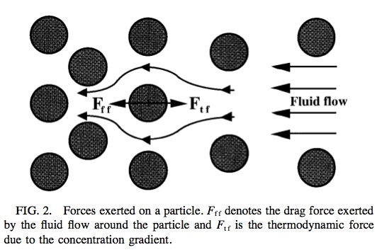
(source ultrafiltration of colloidal dispersions – pdf) I’m going to start by comparing this force balance to the height of the atmosphere.
If you’ll recall (and if you don’t recall, an excellent recap is available on Jim’s website for BME 442), the relative concentration of air in the atmosphere at a height h is given by

where 


where R is the radius of the particle, v is the speed of the fluid, h is the distance from the membrane, and mu is the viscosity. The limiting factor of our previous model was the fact that it used 


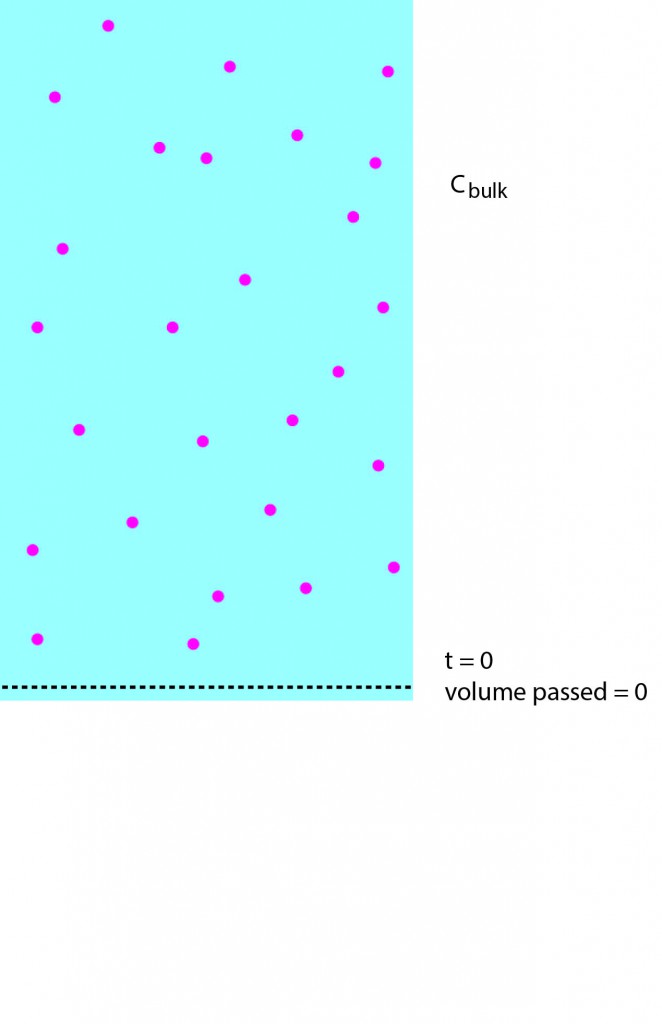
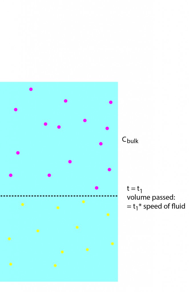
additional gold above membrane = 1-D volume of water passed through the membrane * concentration of feed
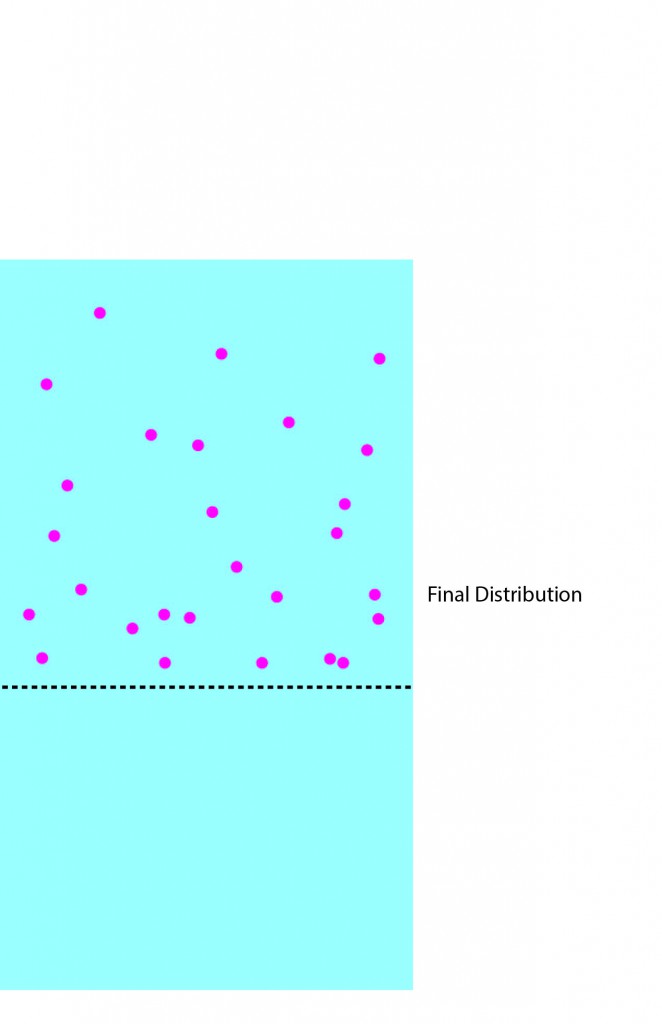
We then note that the 1-D volume of water passed through = v*t (where v is the speed of the fluid and t is the time of separation) , and assume that this gold then instantaneously assumes a boltzmann distribution:

These steps are illustrated in the following sequence of pictures:

I’ve assumed in this case that we can consider the gold that has been rejected to be a separate population from the gold that is still approaching the membrane, which requires some justification. In particular, we assume that the baseline 

while the extra gold is totally stopped and experienced a drag force of

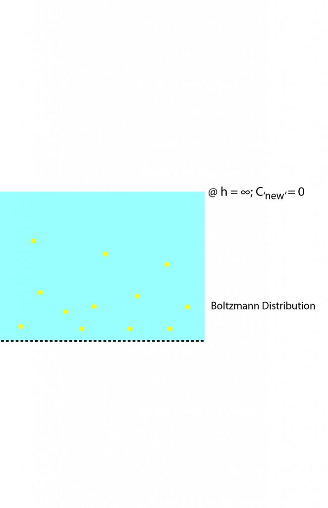
Because at an infinite distance away from the membrane the concentration falls to
Only the gold in excess of

Integrating and simplifying gives us


The concentration at any height would be given by:

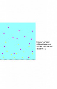
If instead of a perfect membrane that is completely holding back the gold, we have a semi permeable membrane that lets some gold through, the distribution changes to

where 

And here’s another perspective of the system:
The final equations are:
![\langle N \rangle = W\langle V \rangle C_{0} \frac{[1-(C_{\text{filtrate}}/C_{0})e^{-Pe}]}{1-e^{-Pe}} \ \ \ \ (1)](https://s0.wp.com/latex.php?latex=%5Clangle+N+%5Crangle+%3D+W%5Clangle+V+%5Crangle+C_%7B0%7D+%5Cfrac%7B%5B1-%28C_%7B%5Ctext%7Bfiltrate%7D%7D%2FC_%7B0%7D%29e%5E%7B-Pe%7D%5D%7D%7B1-e%5E%7B-Pe%7D%7D+%5C+%5C+%5C+%5C+%281%29&bg=ffffff&fg=000&s=0&c=20201002)


Note that 


The problem with these equations is that they are ‘recursively defined’ (there is a better, proper math word for this characteristic, but I don’t know what it is). By this I mean that N is a function of 
Lets focus this post on the model development only and move the effort to solve it to a second post. There is too much here to digest at once.
Also number your equations. Explain the meaning of each equation along with any new parameters, immediately following the equation.
Karl –
I am trying to follow your logic here, with limited success 🙂
I think that part (all?) of you problem is that you are not including a model of the concentration polarization (cp) ‘layer’ in your overall model. I think this is what you were trying to do at the end of your post.
You should be able to assume steady state in writing the flux eqn in the membrane. You then need to tie this with a flux eqn in the cp layer, which will include an unsteady term. Both of these expressions will include the concentration at the membrane face, and the model of the cp layer can be used to relate this to the bulk feed concentration. But these equations cannot be solved independently.
Here are some papers that you might find helpful:
Zydney, “Stagnant Film Model for Concentration Polarization in Membrane Systems”, JMS vol 130, pp 275-281, 1977.
Kim and Hoek, “Modeling Concentration Polarization in Reverse Osmosis Processes” Desalination, vol 186, pp 111-128, 2005
Trettin and Doshi, “Ultrafiltration in an Unstirred Batch Cell”, Ind. Eng. Chem. Fundam. vol 19, pp. 189-194, 1980.
Balannec and Bariou, “Ultrafiltration and Reverse Osmosis of Small Non-Charged Molecules: A Comparison Study of Rejection in a Stirred and an Unstirred Batch Cell” JMS, vol 164, pp. 141-155, 2000.
The model of the cp layer depends upon the geometry of the cell, and most experiments with UF separations are performed either in a stirred cell or in a plate device with flow normal to the membrane surface. Your device is different than these and so you’ll need to incorporate an appropriate model of your feed chamber in your overall model. The last two papers on my list might help.
I suggest that you focus your model initially on diffusion + convection only. Once you have something that works, then you can add electrostatic interactions to the picture.
Let me know if you want to discuss on the phone. I will be in Rochester more this summer and can let you know when I’ll have some time to meet with you again if that would help.
Ruth