Defining “Resolution” in our Sieving Model
In my earlier posts, as well as in Josh’s NPN paper and Tom’s ACS nano paper, we’ve talked a lot about the resolutions of nanoparticle separations. What we mean by it is how well the membrane is able to discriminate between two similarly sized particles. For instance, we predict that a series of gold nanoparticle filtrations performed at 1.3 PSI using a 6um thick Track etched membrane with 37 nm diameter pores should give a sieving curve like this: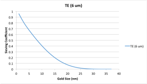
Contrast this with the same separations (1.3 PSI, 37 nm diameter pores) performed with a 50 nm thick NPN/SiN membrane:
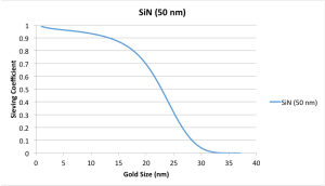
It’s obvious that the NPN membrane is better able to pass 20 nm gold nanoparticles while holding back 30 nm nanoparticles. To quantify this, we came up with a mathematical definition of resolution:

where Δx is the difference between a particle size where 90% of the particles make it through and another particle size where 10% of the particles make it through, and x̄ is the average of the two particle sizes:
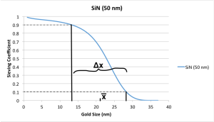
Note that a smaller resolution corresponds to a tighter cutoff and better performance.
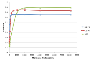
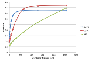
With this definition, I generated the following graph:
Same graph, but ignoring the largest datapoints:
And zooming in still further:
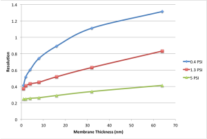
What’s interesting is that from these graphs we expect to see high pressures giving us better resolution for thin membranes (< 200 nm in thickness) but that we will actually expect the opposite behavior for membranes as thick as track etched membranes (6000 nm thick).
This seems a little counterintuitive, so I revisited some of our old data:
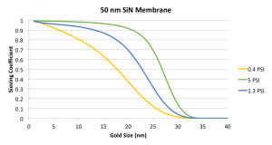
And used the same code to generate the same three curves with a 6um membrane: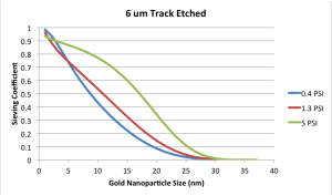
The data seems to agree, at least according to our definition of 90% vs. 10%. I thought maybe if we picked different cutoffs, such as 80% and 20%, we’d see a different ranking, but that doesn’t seem to be the case:
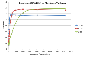
Part of the reason for this shift is that 5 PSI applied to a 6um membrane is very different from 5 PSI applied to a 50 nm membrane. My program runs until 200 uL of fluid passes through the membrane. With a 50 nm membrane, this takes 23 seconds. With a 6 um membrane, this takes 1900 seconds, or ~32 min.
To correct for this, I fixed the flux through the membrane as constant. I chose three different fluxes, corresponding to the fluxes you would get through a 50 nm membrane at 0.4 PSI, 1.3 PSI, and 5 PSI. Again, I calculated the resolution (90/10 resolutions) for a range of thicknesses, but pressure was increased as the membrane got thicker to keep the flux (and therefore the time of separation) constant:
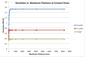
Zoomed in:
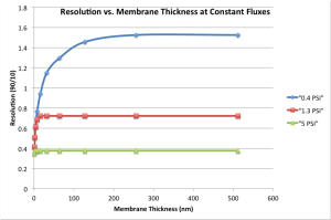
Zoomed in yet more:
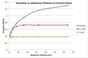
There’s a lot to chew on here.
I think the most difficult graph to explain is the first one in this post – 90/10 resolution vs. membrane thickness at constant pressures:
Why would a higher pressure lead to a higher resolution/broader cutoff/worse performance for very very thick membranes? I think the answer arises from this figure: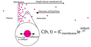
During a separation, the particles adopt a Poisson-Boltzman distribution because of a balance between the Stokes drag towards the membrane and the diffusive flux away from the membrane. But as particle size increases, the Stokes drag increases (linearly) and the diffusion coefficient decreases (linearly). Larger particles experience larger concentration polarizations, then.
The reason that concentration polarization increases fluxes across the membrane is not due to diffusion (except in the case of very thin membranes like graphene, or for particles less than 10 nm in diameter), but due to the fact that the same particle is trying to enter a pore many many times.
Consider a single 20 nm gold nanoparticle above a membrane with 37 nm pores. In a perfectly stirred cell, this particle might hit against the membrane and try to slip through a pore just a single time – in fact, let’s choose the other parameters (pressure, active area) of the separation so that exactly that happens. The probability of the particle passing through just that one time is only 20%. So a perfectly stirred cell would have a sieving coefficient of 0.2 for 20 nm particles.
Now consider the same particle in an unstirred cell with substantial concentration polarization. If the particle does not make it through the first time, the particle doesn’t return to the center of the retentate chamber. Instead, the particle remains just above the surface of the membrane. Now, it interrogates the pore a second time, and if it is rejected, a third time, and so on. Let’s assume that the polarization is enough that a particle interrogates the membrane 3 times on average. Although in the perfectly stirred case, the probability of the particle getting rejected is 80%, in the concentration polarization case the probability of rejection is 0.8*0.8*0.8 = 0.5 = 50% rejection. So the sieving coefficient for the unstirred cell would be 0.5, as contrasted to the sieving coefficient of 0.2 for the stirred cell.
That’s what we’re seeing happen in this case:
Here, the concentration polarization is actually hurting the sieving coefficient, because particles larger than the normal cutoff are being forced through, while the 90% cutoff remains the same.
EDIT
As two final points (and responding to Jim’s comments on the original post) here is the plot of cutoff width Δx vs. membrane thickness. Note that this differs from resolution because the cutoff width is not divided by the average of the two cutoffs, and so both axes of the chart have real units:
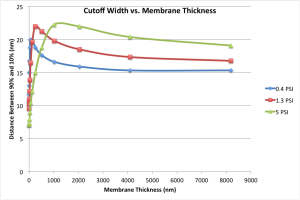
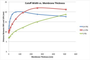
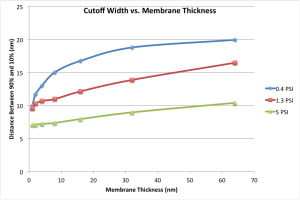
Can you re-plot the ‘resolution’ curves without the normalization please? I’m wondering if the normalization is responsible for some of the cross-over.
The zoomed in curves make the case that higher pressure is required to reach a particular resolution with a thicker membrane
It might also help to see the sieving coefficient as a function of time it should start low and increase as polarization occurs.